Occam’s razor

Many philosophers throughout history have advocated the idea of parsimony. One of the greatest Greek philosophers, Aristotle who goes as far as to say, “Nature operates in the shortest way possible”. It is as a consequence that humans might be biased as well to choose a simpler explanation given a set of all possible explanations with the same descriptive power. This post gives a brief overview of Occam’s razor, the relevance of the principle and ends with a note on the usage of this razor as an inductive bias in machine learning (decision tree learning in particular).

What is Occam’s razor?
Occam’s razor is a law of parsimony popularly stated as (in William’s words) “Plurality must never be posited without necessity”. Alternatively, as a heuristic, it can be viewed as, when there are multiple hypotheses to solve a problem, the simpler one is to be preferred. It is not clear as to whom this principle can be conclusively attributed to, but William of Occam’s (c. 1287 – 1347) preference for simplicity is well documented. Hence this principle goes by the name, “Occam’s razor”. This often means cutting off or shaving away other possibilities or explanations, thus “razor” appended to the name of the principle. It should be noted that these explanations or hypotheses should lead to the same result.

Relevance of Occam’s razor.
There are many events that favor a simpler approach either as an inductive bias or a constraint to begin with. Some of them are :

• Studies like this, where the results have suggested that preschoolers are sensitive to simpler explanations during their initial years of learning and development.
• Preference for a simpler approach and explanations to achieve the same goal is seen in various facets of sciences; for instance, the parsimony principle applied to the understanding of evolution.
• In theology, ontology, epistemology, etc this view of parsimony is used to derive various conclusions.
• Variants of Occam’s razor are used in knowledge Discovery.

Occam’s razor as an inductive bias in machine learning.

Note: It is highly recommended to read the article on decision tree introduction for an insight on decision tree building with examples.

• Inductive bias (or the inherent bias of the algorithm) are assumptions that are made by the learning algorithm to form a hypothesis or a generalization beyond the set of training instances in order to classify unobserved data.
• Occam’s razor is one of the simplest examples of inductive bias. It involves a preference for a simpler hypothesis that best fits the data. Though the razor can be used to eliminate other hypotheses, relevant justification may be needed to do so. Below is an analysis of how this principle is applicable in decision tree learning.
• The decision tree learning algorithms follow a search strategy to search the hypotheses space for the hypothesis that best fits the training data. For example, the ID3 algorithm uses a simple to complex strategy starting from an empty tree and adding nodes guided by the information gain heuristic to build a decision tree consistent with the training instances.
  The information gain of every attribute (which is not already included in the tree) is calculated to infer which attribute to be considered as the next node. Information gain is the essence of the ID3 algorithm. It gives a quantitative measure of the information that an attribute can provide about the target variable i.e, assuming only information of that attribute is available, how efficiently can we infer about the target. It can be defined as :



• Well, there can be many decision trees that are consistent with a given set of training examples, but the inductive bias of the ID3 algorithm results in the preference for simper (or shorter trees) trees. This preference bias of ID3 arises from the fact that there is an ordering of the hypotheses in the search strategy. This leads to additional bias that attributes high with information gain closer to the root is preferred. Therefore, there is a definite order the algorithm follows until it terminates on reaching a hypothesis that is consistent with the training data.



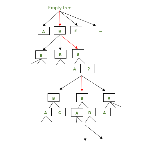
The above image depicts how the ID3 algorithm chooses the nodes in every iteration. The red arrow depicts the node chosen in a particular iteration while the black arrows suggest other decision trees that could have been possible in a given iteration.

• Hence starting from an empty node, the algorithm graduates towards more complex decision trees and stops when the tree is sufficient to classify the training examples.
• This example pops a question. Does eliminating complex hypotheses bear any consequence on the classification of unobserved instances? simply put, does the preference for a simpler hypothesis have an advantage? If two decision trees have slightly different training errors but the same validation errors, then it is obvious that the simpler tree among the two will be chosen. As a higher validation error causes overfitting of the data. Complex trees often have almost zero training error, but the validation errors might be high. This scenario gives a logical reason for a bias towards simpler trees. In addition to that, a simpler hypothesis might prove effective in a resource-limited environment.
• What is overfitting? Consider two hypotheses a and b. Let ‘a’ fit the training examples perfectly, while the hypothesis ‘b’ has a small training error. If over the entire set of data (i.e, including the unseen instances), if the hypothesis ‘b’ performs better, then ‘a’ is said to overfit the training data. To best illustrate the problem of over-fitting, consider the figure below.

  

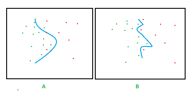
  Figures A and B depict two decision boundaries. Assuming the green and red points represent the training examples, the decision boundary in B perfectly fits the data thus perfectly classifying the instances, while the decision boundary in A does not, though being simpler than B. In this example the decision boundary in B overfits the data. The reason being that every instance of the training data affects the decision boundary. The added relevance is when the training data contains noise. For example, assume in figure B that one of the red points close to the boundary was a noise point. Then the unseen instances in close proximity to the noise point might be wrongly classified. This makes the complex hypothesis vulnerable to noise in the data.

• While the problem of overfitting behaviour of a model can be significantly avoided by settling for a simpler hypothesis, an extremely simple hypothesis may be too abstract to deduce any information needed for the task resulting in underfitting. Overfitting and underfitting are one of the major challenges to be addressed before we zero in on a machine learning model. Sometimes a complex model might be desired, it’s a choice dependent on the data available, the results expected and the application domain.

Note: For additional information on the decision tree learning, please refer to Tom M. Mitchell’s “Machine Learning” book.