Understanding Nonlinear Regression with Examples

In this article, we will see some examples of non-linear regression in machine learning that are generally used in regression analysis, the reason being that most of the real-world data follow highly complex and non-linear relationships between the dependent and independent variables.

Non-linear regression in Machine Learning

Nonlinear regression refers to a broader category of regression models where the relationship between the dependent variable and the independent variables is not assumed to be linear. If the underlying pattern in the data exhibits a curve, whether it’s exponential growth, decay, logarithmic, or any other non-linear form, fitting a nonlinear regression model can provide a more accurate representation of the relationship. This is because in linear regression it is pre-assumed that the data is linear. 

A nonlinear regression model can be expressed as:

Where,

•  : Regression function
• X: This is the vector of independent variables, which are used to predict the dependent variable.
• :The vector of parameters that the model aims to estimate. These parameters determine the shape and characteristics of the regression function.
• : error term

Many different regressions exist and can be used to fit whatever the dataset looks like such as quadratic, cubic regression, and so on to infinite degrees according to our requirement.

Assumptions in NonLinear Regression

These assumptions are similar to those in linear regression but may have nuanced interpretations due to the nonlinearity of the model. Here are the key assumptions in nonlinear regression:

1. Functional Form: The chosen nonlinear model correctly represents the true relationship between the dependent and independent variables.
2. Independence: Observations are assumed to be independent of each other.
3. Homoscedasticity: The variance of the residuals (the differences between observed and predicted values) is constant across all levels of the independent variable.
4. Normality: Residuals are assumed to be normally distributed.
5. Multicollinearity: Independent variables are not perfectly correlated.

Types of Non-Linear Regression

There are two main types of Non Linear regression in Machine Learning:

1. Parametric non-linear regression assumes that the relationship between the dependent and independent variables can be modeled using a specific mathematical function. For example, the relationship between the population of a country and time can be modeled using an exponential function. Some common parametric non-linear regression models include: Polynomial regression, Logistic regression, Exponential regression, Power regression etc.
2. Non-parametric non-linear regression does not assume that the relationship between the dependent and independent variables can be modeled using a specific mathematical function. Instead, it uses machine learning algorithms to learn the relationship from the data. Some common non-parametric non-linear regression algorithms include: Kernel smoothing, Local polynomial regression, Nearest neighbor regression etc.

Non-Linear Regression Algorithms

Nonlinear regression encompasses various types of models that capture relationships between variables in a nonlinear manner. Here are some common types:

Polynomial Regression

Polynomial regression is a type of nonlinear regression that fits a polynomial function to the data. The general form of a polynomial regression model is:

where,

• y : dependent variable
• X : independent variable
• : parameters of the model
• n : degree of the polynomial

Exponential Regression

Exponential regression is a type of nonlinear regression that fits an exponential function to the data. The general form of an exponential regression model is:

where,

• y – dependent variable
• X – independent variable
• – parameters of the model

Logarithmic Regression

Logarithmic regression is a type of nonlinear regression that fits a logarithmic function to the data. The general form of a logarithmic regression model is:

where,

• y – dependent variable
• X – independent variable
• – parameters of the model

Power Regression

Power regression is a type of nonlinear regression that fits a power function to the data. The general form of a power regression model is:

where,

• y – dependent variable
• X – independent variable
• – parameters of the model

Generalized Additive Models (GAMs)

Generalized additive models (GAMs) are a type of nonlinear regression that combines multiple linear models to model a complex relationship between variables. The general form of a GAM is:

where,

• y – dependent variable
• x1, x2,….,xn – independent variable
• f1(x1), f2(x2), …, fn(xn) – smooth functions of the independent variables
• – error term

Gauss-Newton Algorithm:

The Gauss-Newton algorithm is an iterative optimization method designed for minimizing the sum of squared differences between observed and predicted values in nonlinear least squares regression. It iteratively updates parameter estimates by moving in the direction of the gradient of the objective function, leveraging the Jacobian matrix and the residuals.

Gradient Descent algorithm

The Gradient Descent algorithm is a widely used iterative optimization technique for finding the minimum of a function. In the context of nonlinear regression, it updates parameter estimates by iteratively moving towards the direction of the steepest decrease in the objective function, with the learning rate controlling the step size.

Levenberg-Marquardt algorithm

The Levenberg-Marquardt algorithm is a modification of the Gauss-Newton algorithm that introduces a damping parameter to enhance robustness. It dynamically adjusts the step size during iterations by combining the advantages of Gauss-Newton and gradient descent methods, providing a versatile approach for solving nonlinear least squares problems.

Evaluating Non-Linear Regression Models

Evaluating the performance of a nonlinear regression model is crucial to ensure it accurately represents the underlying relationship between the independent and dependent variables.

There are a number of different metrics that can be used to evaluate non-linear regression models, but some common metrics are:

1. R-squared – R-squared (Coefficient of Determination) measures the proportion of variance in the dependent variable that is explained by the independent variables in the model. It ranges from 0 to 1, where 0 indicates no explanation of variance and 1 indicates perfect explanation. A higher R-squared value suggests a better model fit.
2. Adjusted R-squared – Adjusted R-squared is a modified version of R-squared that accounts for the number of independent variables in the model. It penalizes models with more variables, making it a more appropriate measure of goodness of fit when comparing models with different numbers of independent variables. A higher adjusted R-squared value indicates a better model fit.
3. Root Mean Squared Error (RMSE) – Root Mean Squared Error (RMSE) is the square root of MSE, providing a more intuitive measure of the average error in predictions. It represents the average distance between the predicted and actual values of the dependent variable, scaled to the same units as the dependent variable. A lower RMSE signifies a better model fit.

How does a Non-Linear Regression work?

Non-linear regression algorithms work by iteratively adjusting the parameters of a non-linear function to minimize the error between the predicted values of the dependent variable and the actual values. The specific function used depends on the nature of the relationship between the variables, and there are many different types of non-linear functions that can be used.

• If we observe closely then we will realize that to evolve from linear regression to non-linear regression. We are just supposed to add the higher-order terms of the dependent features in the feature space. This is sometimes also known as feature engineering but not exactly.
• The addition of non-linear terms is what allows us to fit a curvilinear model to the data at hand. Even though the non-linear regression is similar to the linear one but the different types of challenges are faced by the Machine Learning practitioner while training such a model. And hence several established methods, such as Levenberg-Marquardt and Gauss-Newton, are used to develop nonlinear models.

Here we are implementing Non-Linear Regression using Python:

Step-1: Importing libraries

Importing all the necessary libraries:

Python3

import pandas as pd
import numpy as np
import matplotlib.pyplot as plt
from sklearn.preprocessing import PolynomialFeatures
from sklearn.linear_model import LinearRegression
from sklearn.metrics import mean_absolute_error, mean_squared_error, r2_score

Step-2: Import Dataset

Importing and reading the dataset: Dataset Link

Python3

# Read the CSV file
df = pd.read_csv('/content/gdp.csv')

# Display the first few rows of the dataframe
print(df.head())

Output:

Year         Value
0  1960  5.918412e+10
1  1961  4.955705e+10
2  1962  4.668518e+10
3  1963  5.009730e+10
4  1964  5.906225e+10

Plot the Original Gdp

Creates a scatter plot of the Year (independent variable) vs. Value (dependent variable).

Python3

plt.figure(figsize=(8, 5))
x_original, y_original = df["Year"].values, df["Value"].values
plt.plot(x_original, y_original, 'bo')
plt.ylabel('GDP')
plt.xlabel('Year')
plt.title('Original GDP Data')
plt.show()

Output:

Simple logistic model curve

Representing a simple logistic model curve over a range of independent variable values.

Python3

#Plot a simple logistic model curve
X_logistic = np.arange(-5.0, 5.0, 0.1)
Y_logistic = 1.0 / (1.0 + np.exp(-X_logistic))

plt.plot(X_logistic, Y_logistic, color='green')  # Orange color for the logistic curve
plt.ylabel('Dependent Variable')
plt.xlabel('Independent Variable')
plt.title('Simple Logistic Model Curve')
plt.show()

Output:

Define Sigmoid Function

• Implements the sigmoid function (logistic function) that maps any real number to a value between 0 and 1.
• Takes two parameters: Beta_1 (slope) and Beta_2 (intercept).
• Assigns initial values for Beta_1 and Beta_2 based on intuition or estimation.
• Applies the sigmoid function to the original data with the initial parameter values.

Python3

#Define the sigmoid function
def sigmoid(x, Beta_1, Beta_2):
    y = 1 / (1 + np.exp(-Beta_1 * (x - Beta_2)))
    return y

# Set initial values for logistic function parameters
beta_1_initial = 0.10
beta_2_initial = 1990.0

#Apply logistic function to the data
Y_pred_logistic = sigmoid(x_original, beta_1_initial, beta_2_initial)

Plot the initial prediction against datapoints

Plots the predicted values (scaled up by 15000000000000 for better visibility) compared to the actual data points.

Python3

plt.plot(x_original, Y_pred_logistic * 15000000000000., color='purple', label='Initial Prediction')
plt.plot(x_original, y_original, 'go', label='Data')
plt.ylabel('GDP')
plt.xlabel('Year')
plt.legend()
plt.title('Initial Logistic Regression Fit')
plt.show()

Output:

Normalizing Data

• Divides both Year and Value by their respective maximum values to scale them between 0 and 1.

Python3

# Normalize the data
x_normalized = x_original / max(x_original)
y_normalized = y_original / max(y_original)

Fitting sigmoid function to normalized data

• Uses the curve_fit function from scipy.optimize to find the best-fitting parameters for the sigmoid function based on the normalized data.
• Returns the optimal parameters (popt) and their covariance matrix (pcov).
• Prints the optimized values of Beta_1 and Beta_2 found by the curve fitting.

Python3

from scipy.optimize import curve_fit
# Fit the sigmoid function to the normalized data
popt, pcov = curve_fit(sigmoid, x_normalized, y_normalized)

# Print the final parameters
print("Beta_1 = %f, Beta_2 = %f" % (popt[0], popt[1]))

Output:

Beta_1 = 690.451709, Beta_2 = 0.997207

Normalized Sigmoid Regression

1. Defining a new x range for the fitted curve
   • Creates a new range of Year values within the original data range for plotting the fitted curve.
2. Applying the fitted sigmoid function
   • Applies the sigmoid function to the new Year range using the optimized parameters from step 10.
3. Plotting the normalized data and fitted curve:
   • Plots the normalized data points, the fitted sigmoid curve, and a legend.
   • Shows the improved fit after optimization compared to the initial prediction.

Python3

# Create a new x range for the fitted sigmoid curve
x_fit = np.linspace(1960, 2015, 55) / max(x_original)

# Apply the sigmoid function with the fitted parameters
y_fit = sigmoid(x_fit, *popt)

# Plot the normalized data, the sigmoid fit, and the legend
plt.figure(figsize=(8, 5))
plt.plot(x_normalized, y_normalized, 'go', label='Normalized Data')  # Changed color to green for data points
plt.plot(x_fit, y_fit, linewidth=3.0, color='purple', label='Sigmoid Fit')  # Changed color to purple for the sigmoid fit line
plt.legend(loc='best')
plt.ylabel('GDP')
plt.xlabel('Year')
plt.title('Normalized Sigmoid Regression Fit')
plt.show()

Output:

Predictions

1. Splitting data into train/test sets: Randomly splits the normalized data and target values into separate training and testing sets (80% and 20% respectively).
2. Building the model with the train set: Applies the curve_fit function again to find the best-fitting parameters for the sigmoid function using only the training data.
3. Predicting with the test set: Applies the model learned from the training data (using the trained parameters) to the test set to predict the normalized target values.
4. Evaluating the model:
   • Calculates three evaluation metrics: mean absolute error (MAE), mean squared error (MSE), and R-squared.
   • These metrics measure the difference between the predicted and actual values and the model’s goodness of fit.

Python3

#Split data into train/test sets
random_mask = np.random.rand(len(df)) < 0.8
train_x = x_normalized[random_mask]
test_x = x_normalized[~random_mask]
train_y = y_normalized[random_mask]
test_y = y_normalized[~random_mask]

#Build the model using the train set
popt_train, pcov_train = curve_fit(sigmoid, train_x, train_y)

#Predict using the test set
y_hat_test = sigmoid(test_x, *popt_train)

#Evaluate the model
mae = mean_absolute_error(test_y, y_hat_test)
mse = np.mean((y_hat_test - test_y) ** 2)
r2 = r2_score(y_hat_test, test_y)

#Print the evaluation metrics
print("Mean Absolute Error: %.2f" % mae)
print("Mean Squared Error: %.2f" % mse)
print("R2-score: %.2f" % r2)

Output:

Mean absolute error: 0.05
Residual sum of squares (MSE): 0.00
R2-score: 0.88

Considerations:

For a model to be considered non-linear, Y hat must be a non-linear function of the parameters Theta, not necessarily the features X. When it comes to the non-linear equation, it can be the shape of exponential, logarithmic, logistic, or many other types. 

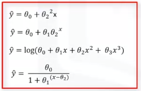
Non-Linear Regression Equations

As you can see in all of these equations, the change of Y hat depends on changes in the parameters Theta, not necessarily on X only. That is, in non-linear regression, a model is non-linear by parameters.

Linear VS Non-Linear Regression

Feature	Linear Regression	Non Linear Regression
Relationship between variables	Assumes a linear relationship between the independent and dependent variables	Allows for non-linear relationships between the independent and dependent variables
Model complexity	Simpler model with fewer parameters	More complex model with more parameters
Interpretability	Highly interpretable due to the linear relationship	Less interpretable due to the non-linear relationship
Overfitting susceptibility	More susceptible to overfitting due to its simplicity	Less susceptible to overfitting due to its ability to capture complex relationships
Flexibility	Requires large datasets to accurately estimate the linear relationship	Can work with smaller datasets due to its flexibility
Applications	Suitable for predicting continuous target variables when the relationship is linear	Suitable for predicting continuous target variables when the relationship is non-linear
Examples	Predicting house prices based on size and location	Predicting customer churn based on behavioral patterns

Applications of Non-Linear Regression

As we know that most of the real-world data is non-linear and hence non-linear regression techniques are far better than linear regression techniques. Non-Linear regression techniques help to get a robust model whose predictions are reliable and as per the trend followed by the data in history. Tasks related to exponential growth or decay of a population, financial forecasting, and logistic pricing model were all successfully accomplished by the Non-Linear Regression techniques.

1. The insurance industry makes use of it. Its application is seen, for instance, in the IBNR reserve computation.
2. In the field of agricultural research, it is crucial. Considering that nonlinear models more accurately represent numerous crops and soil dynamics than linear ones.
3. There are uses for nonlinear models in forestry research because the majority of biological processes are inherently nonlinear. An example would be a straightforward power function that relates a tree’s weight or volume to its height or diameter.
4. It is employed in the framing of the problem and the derivation of statistical solutions to the calibration problem in research and development.
5. One example from the world of chemistry is the development of a wide-range colorless gas, HCFC-22 formulation, using a nonlinear model.

Advantages & Disadvantages of Non-Linear Regression

Advantages of Non-Linear Regression

1. Non-linear regression can model relationships that are not linear in nature.
2. Non-linear regression can be used to make predictions about the dependent variable based on the values of the independent variables.
3. Non-linear regression can be used to identify the factors that influence the dependent variable.

Disadvantages of Non-Linear Regression

1. Non-linear regression models can be more complex to implement than linear regression.
2. Non-linear regression models can be more sensitive to outliers than linear regression models.
3. Non-linear regression models can be more computationally expensive to train than linear regression models.

Conclusion

Non-linear regression using Python is a powerful tool for modeling relationships that are not linear in nature. It is used in a wide variety of fields, including economics, finance, medicine, science, and engineering.

Non-linear regression can be a complex topic, but it is worth learning if you need to model relationships that are not linear in nature.

Frequently Asked Questions (FAQs) on Non-Linear Regression

1. What is non-linear regression?

Non-linear regression in Machine Learning is a statistical method used to model the relationship between a dependent variable and one or more independent variables when that relationship is not linear. This means that the relationship between the variables cannot be represented by a straight line.

2. Is nonlinear regression better than linear regression?

• Non-linear regression is more flexible than linear regression and can model a wider range of relationships between variables.
• Non-linear regression can be more accurate than linear regression for nonlinear relationships.
• Non-linear regression is more complex and computationally expensive than linear regression.
• The choice between linear and non-linear regression depends on the specific problem and data.

3. How do you calculate nonlinear regression?

Calculating Non Linear Regression using Python involves fitting a nonlinear model to the data to capture the relationship between the dependent and independent variables.

Can be calculated using

Where,

• f – Regression function
• (X,β) – vector parameters
• – error term

4. When should I use non-linear regression?

You should use Non Linear Regression in Machine Learning when the relationship between the dependent and independent variables is not linear. This can be determined by plotting the data and inspecting the scatterplot.