Noise Removal using Lowpass Digital Butterworth Filter in Scipy – Python
Last Updated :
13 Jan, 2021
In this article, the task is to write a Python program for Noise Removal using Lowpass Digital Butterworth Filter.
What is the noise?
Noise is basically the unwanted part of an electronic signal. It is often generated due to fault in design, loose connections, fault in switches etc.
What to do if we have noise in our signal?
To remove unwanted signals/noise we use filters of different types and specifications. Generally in the industry we need to choose the best fit by testing it with the signal to pinpoint the best filter to be used for removing the noise in a given use case.
What are we going to do now?
We are going to implement a Lowpass Digital Butterworth Filter now to remove the unwanted signal/noise of a combination of sinusoidal waves.
Filter Specifications:
- Signal made up of 25 Hz and 50 Hz
- Sampling frequency 1kHz.
- Order N=10 at 35Hz to remove 50Hz tone.
Step by Approach:
Step 1:Importing the libraries
Python3
import numpy as np
import scipy.signal as signal
import matplotlib.pyplot as plt
|
Step 2:Defining the specifications
Python3
f1 = 25
f2 = 50
N = 10
t = np.linspace(0, 1, 1000)
sig = np.sin(2*np.pi*f1*t) + np.sin(2*np.pi*f2*t)
|
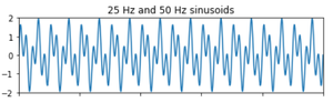
Step 3:Plot the original signal with noise
Python3
fig, (ax1, ax2) = plt.subplots(2, 1, sharex=True)
ax1.plot(t, sig)
ax1.set_title('25 Hz and 50 Hz sinusoids')
ax1.axis([0, 1, -2, 2])
sos = signal.butter(50, 35, 'lp', fs=1000, output='sos')
|
Output:
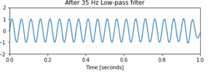
Step 4:Plot of the signal after removing noise
Python3
filtered = signal.sosfiltfilt(sos, sig)
ax2.plot(t, filtered)
ax2.set_title('After 35 Hz Low-pass filter')
ax2.axis([0, 1, -2, 2])
ax2.set_xlabel('Time [seconds]')
plt.tight_layout()
plt.show()
|
Output:
Step 5: Implementation
Python3
import numpy as np
import scipy.signal as signal
import matplotlib.pyplot as plt
f1 = 25
f2 = 50
N = 10
t = np.linspace(0, 1, 1000)
sig = np.sin(2*np.pi*f1*t) + np.sin(2*np.pi*f2*t)
fig, (ax1, ax2) = plt.subplots(2, 1, sharex=True)
ax1.plot(t, sig)
ax1.set_title('25 Hz and 50 Hz sinusoids')
ax1.axis([0, 1, -2, 2])
sos = signal.butter(50, 35, 'lp', fs=1000, output='sos')
filtered = signal.sosfiltfilt(sos, sig)
ax2.plot(t, filtered)
ax2.set_title('After 35 Hz Low-pass filter')
ax2.axis([0, 1, -2, 2])
ax2.set_xlabel('Time [seconds]')
plt.tight_layout()
plt.show()
|
Output:
Like Article
Suggest improvement
Share your thoughts in the comments
Please Login to comment...