Natural Cubic spline
Last Updated :
18 Jul, 2021
Cubic Spline:
The cubic spline is a spline that uses the third-degree polynomial which satisfied the given m control points. To derive the solutions for the cubic spline, we assume the second derivation 0 at endpoints, which in turn provides a boundary condition that adds two equations to m-2 equations to make them solvable. The system of equations for the Cubic spline for 1-dimension can be given by:

We take a set of points [xi, yi] for i = 0, 1, …, n for the function y = f(x). The cubic spline interpolation is a piecewise continuous curve, passing through each of the values in the table.
- Following are the conditions for the spline of degree K=3:
- The domain of s is in intervals of [a, b].
- S, S’, S” are all continuous function on [a,b].
![S(x) =\begin{bmatrix} S_0 (x), x \epsilon [x_0, x_1] \\ S_1 (x), x \epsilon [x_1, x_2] \\ ... \\ ... \\ ... \\ S_{n-1} (x), x \epsilon [x_1, x_2] \end{bmatrix}](https://www.geeksforgeeks.org/wp-content/ql-cache/quicklatex.com-bfe0b4a8fddd8d349888f0eb303f7f44_l3.png "Rendered by QuickLaTeX.com")
Here Si(x) is the cubic polynomial that will be used on the subinterval [xi, xi+1].
Since, there are n intervals and 4 coefficients of each equation, for that we require a 4n parameters to solve the spline, we can get 2n equation from the fact that each of the cubic spline equation should satisfy the value at both ends:

The above cubic spline equations should not only continuous and differentiable but also have defined first and second derivatives that are also continuous on control points.

and

For 1, 2, 3…n-1 provides the 2n -2 equation constraints. So, we need 2 more equations to solve the above cubic spline. For that, we will use some natural boundary conditions.
Natural Cubic Spline:
In Natural cubic spline, we assume that the second derivative of the spline at boundary points is 0:

Now, since the S(x) is a third-order polynomial we know that S”(x) is a linear spline which interpolates. Hence, first, we construct S”(x) then integrate it twice to obtain S(x).
Now, let’s assume t_i = x_i for i= 0, 1,…n, and  and from the natural boundary condition
  . Twice differentiating a cubic spline gives a linear spline which can be written as:

where,

Now, the equation becomes:

Integrating this equation two times to obtain the cubic spline:

where,

Now, to check for the continuity of derivative at t_i i.e S^{‘}_{i}(t_i) = S^{‘}_{i-1}(t_{i}). We first need to find derivatives and put that condition:

where,

Putting the above equation for the continuity and solving it gives the following equation:

Take, v_i = 6(b_i – b_{i-1}) and the above equation can be written as form of matrix:

Implementation
- In this implementation, we will be performing the spline interpolation for function f(x) = 1/x for points b/w 2-10 with cubic spline that satisfied natural boundary condition.
Python3
import matplotlib.pyplot as plt
import numpy as np
from scipy.interpolate import CubicSpline, interp1d
plt.rcParams['figure.figsize'] =(12,8)
x = np.arange(2,10)
y = 1/(x)
cs = CubicSpline(x, y, extrapolate=True)
ns = CubicSpline(x, y,bc_type='natural', extrapolate=True)
linear_int = interp1d(x,y)
xs = np.arange(2, 9, 0.1)
ys = linear_int(xs)
plt.plot(x, y,'o', label='data')
plt.plot(xs,ys, label="interpolation", color='green')
plt.legend(loc='upper right', ncol=2)
plt.title('Linear Interpolation')
plt.show()
xs = np.arange(1,15)
plt.plot(x, y, 'o', label='data')
plt.plot(xs, 1/(xs), label='true')
plt.plot(xs, cs(xs), label="S")
plt.plot(xs, ns(xs), label="NS")
plt.plot(xs, ns(xs,2), label="NS''")
plt.plot(xs, ns(xs,1), label="NS'")
plt.legend(loc='upper right', ncol=2)
plt.title('Cubic/Natural Cubic Spline Interpolation')
plt.show()
print("Value of double differentiation at boundary conditions are %s and %s"
%(ns(2,2),ns(10,2)))
|
Output:
Value of double differentiation at boundary conditions are -1.1102230246251565e-16 and -0.00450262550915248
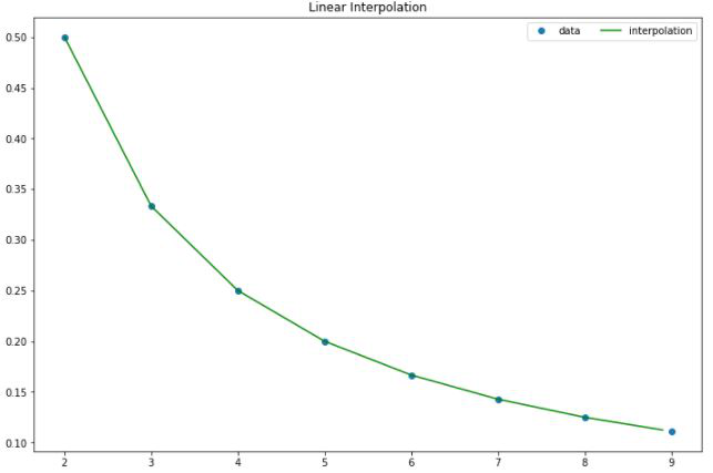
Linear Interpolation
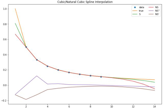
Cubic/Natural Spline Interpolation
References:
Like Article
Suggest improvement
Share your thoughts in the comments
Please Login to comment...