Named Range in Excel

Last Updated : 09 Nov, 2022

We can use the name for the cell Ranges instead of the cell reference (such as A1 or A1:A10). We can create a named range for a range of cells and use then use that name directly in the Excel formulas. When we have huge data sets, Excel-named ranges make it easy to refer (by directly using a name to that data set).

Creating an Excel Named Range :

There can be 3 ways to create named ranges in Excel :

Method 1: Using Define Name

Use the following steps to create named range using Define Name :

Select the range B1:B5.
Click on the Formulas tab.
Then click on Define Name.

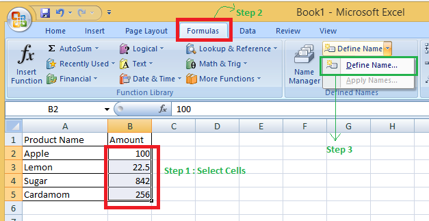
Give a new Name(PriceTotal in our example) & click Ok. (You can see the range in the bottom refers to section, here absolute referencing is used, $ before the row number/ column letter locks the row/column).

Now, the next thing is to see that how to use this named range in any of the Excel formulas. For example, if you want to get the sum of all numbers in the above name range then, can say simply write: =SUM(PriceTotal).

Here, B7 =SUM(PriceTotal) = 100 + 22.5 + 843 + 256 (all the numbers in the named range)= 1220.5

Note: The named Range created by this method is restricted to a worksheet.

Method 2: Use the Name Box

Use the following steps to create a named range using the name box :

Choose the range for which you’d want to give it a name (not the headers).
Type the name of the range with which you wish to construct the Named Range in the Name Box on the left of the Formula bar.

Note: The Name created this way is available in the entire excel current Workbook.

Method 3: From Selection Option

When you have tabular data and wish to construct named ranges for each column/row, this is the preferred method.

Example: We have 3 columns having headers: Product Name, Amount & Tax Percent.

Use the following steps to create a named range from the selection option :

Select the complete data set (the 3 columns with the headers).
Click on the Formulas tab.
Click Create from Selection (or press Control + Shift + F3).

After the click, Create Names from Selection’ dialogue box will be opened.

Check the settings where you have the headers in the Create Names from Selection dialogue box. Because the heading is in the top row, we only select the top row. You can choose both if you have headers in the top row and left column. We only need to check the Left Column option, if the data is organized with the headers only in the left column.

Here we select only Top row because we have headers in the top row.

Result: The data set you selected in column A will be having a named Range: Product_Name (Spaces not allowed, so underscore automatically replaces space)

The data set you selected in column B will be having a named Range: Amount

The data set you selected in column C will be having a named Range: TAX_Percent (Spaces not allowed, so underscore automatically replaces space)

Benefits of Creating Named Ranges in Excel:

The following are benefits of creating & use Named Ranges in Excel :

Instead of using cell references every time, we can directly use Named Reference

Example 1: In the above example, to calculate the sum, we used B7 =SUM(PriceTotal) instead of B7 = SUM(B2:B5) for the above data range.

Example 2: If for the same-named Range, if we write, B9 = SUMIF(PriceTotal,”>50″), then the sum will be equal to the sum of all numbers > 50 in the named range.

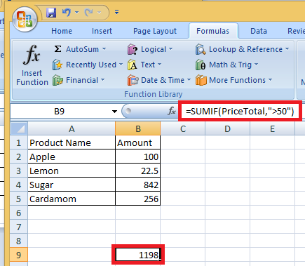
Here, sum is done for all the numbers > 50 in the named range “PriceTotal” = 100+842+256 = 1198.

To Select Cells, you do not need to return to the data set to choose the cells. You can directly use the Named range, by typing the first few characters of the named range, excel shows a list of named ranges that matches the typed characters.

Example :

As you can see that after just typing Pr, a drop-down list for the available options(formula & named Range) is pooped up.

The formulas become dynamic using named Ranges:
- Excel formulas become dynamic if we use Named Ranges. In the above example, if we add another cell of Tax Percent (2.5%)& you name it as “TAX” . Now to calculate Final Price (including tax), we can use the Named Range instead of using the value 2.5.
- Now, if later tax is increased to 3%, you just have to update the Named Range, and all the calculations would be done automatically & we will get the Final Price according to the latest tax percent.
Finding a named cell is less time-consuming.

Using Create From Selection Option :

When generating Named Ranges in Excel, you should be aware of the following naming conventions:

A letter and underscore character(_), or a backslash, shall be the initial character in a Named Range (\). It will display an error if it is anything else is used. Letters, numbers, special characters, a period, or an underscore can make up the remaining characters.
When establishing named ranges, you can’t use spaces. Tax Percent, for example, cannot be a named range. We can use an underscore, a period, or capital characters if we wish to make a Named Range out of two words, You may, for example, Tax_Percent, TaxPercent, etc.
In Excel, you can’t use names that are also cell references. You can’t use C1 because it’s also a cell reference.
You can only have a maximum of 255 characters in a named range.
For Excel, uppercase and lowercase letters are the same when generating named ranges. For example, if you create a named range called ‘TAX’, you cannot create another named range called ‘Tax’ or ‘tax’.

Name Rows and Columns in Excel:

You may find yourself producing a lot of Named Ranges in Excel when working with large data sets and complex models. It is possible that you can’t recall the name of the Named Range you made. What to do then?