Multivariate Optimization – Gradient and Hessian

Last Updated : 24 Sep, 2021

In a multivariate optimization problem, there are multiple variables that act as decision variables in the optimization problem.
z = f(x₁, x₂, x₃…..x_n)

So, when you look at these types of problems a general function z could be some non-linear function of decision variables x₁, x₂, x₃ to x_n. So, there are n variables that one could manipulate or choose to optimize this function z. Notice that one could explain univariate optimization using pictures in two dimensions that is because in the x-direction we had the decision variable value and in the y-direction, we had the value of the function. However, if it is multivariate optimization then we have to use pictures in three dimensions and if the decision variables are more than 2 then it is difficult to visualize.

Gradient:
Before explaining gradient let us just contrast with the necessary condition of univariate case. So in case of uni-variate optimization the necessary condition for x to be the minimizer of the function f(x) is:
First-order necessary condition: f'(x) = 0

So, the derivative in a single-dimensional case becomes what we call as a gradient in the multivariate case.

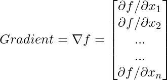
According to the first-order necessary condition in univariate optimization e.g f'(x) = 0 or one can also write it as df/dx. However, since there are many variables in the case of multivariate and we have many partial derivatives and the gradient of the function f is a vector such that in each component one can compute the derivative of the function with respect to the corresponding variable. So, for example, $\partial f/ \partial x_1$ is the first component, $\partial f/ \partial x_2$ is the second component and $\partial f/ \partial x_n$ is the last component.
$Gradient = \nabla f = \begin{bmatrix} \partial f/ \partial x_1\\ \partial f/ \partial x_2\\ ...\\ ...\\ \partial f/ \partial x_n\\ \end{bmatrix}$

Note: Gradient of a function at a point is orthogonal to the contours.

Hessian:
Similarly in case of uni-variate optimization the sufficient condition for x to be the minimizer of the function f(x) is:
Second-order sufficiency condition: f”(x) > 0 or d²f/dx² > 0

And this is replaced by what we call a Hessian matrix in the multivariate case. So, this is a matrix of dimension n*n, and the first component is $\partial ^2f/ \partial x_1^2$ , the second component is $\partial ^2f/\partial x_1 \partial x_2$ and so on.

$Hessian = \nabla ^2 f = \begin{bmatrix} \partial ^2f/ \partial x_1^2 & \partial ^2f/\partial x_1 \partial x_2 & ... & \partial ^2f/ \partial x_1 \partial x_n\\ \partial ^2f/\partial x_2 \partial x_1 & \partial ^2f/ \partial x_2^2 & ... & \partial ^2f/ \partial x_2 \partial x_n\\ ... & ... & ... & ...\\ ... & ... & ... & ...\\ \partial ^2f/\partial x_n \partial x_1 & \partial ^2f/\partial x_n \partial x_2 & ... & \partial ^2f/ \partial x_n^2\\ \end{bmatrix}$

Note:

Hessian is a symmetric matrix.
Hessian matrix is said to be positive definite at a point if all the eigenvalues of the Hessian matrix are positive.

Suggest improvement

Challenges and Problems in Data Cleaning

Solving Linear Regression in Python

Share your thoughts in the comments

Multivariate Optimization – Gradient and Hessian

Please Login to comment...

Similar Reads

What kind of Experience do you want to share?