Moore – Penrose Pseudoinverse | Mathematics

Last Updated : 03 Oct, 2019

In linear algebra pseudoinverse ( $A^{+}$ ) of a matrix A is a generalization of the inverse matrix. The most common use of pseudoinverse is to compute the best fit solution to a system of linear equations which lacks a unique solution. Moore – Penrose inverse is the most widely known type of matrix pseudoinverse. The term generalized inverse is sometimes used as a synonym of pseudoinverse. Let the system is given as: $\overrightarrow{y} = A\overrightarrow{x}$ We know A and $\overrightarrow{y}$ , and we want to find $\overrightarrow{x}$ . Where: $\overrightarrow{x}$ and $\overrightarrow{y}$ are vectors, A is a matrix If A is a square matrix, we proceed as below: $\overrightarrow{y} = A\overrightarrow{x}$ $A^{-1}\overrightarrow{y} = A^{-1}A\overrightarrow{x}$ $A^{-1}\overrightarrow{y} = I\overrightarrow{x}$ $A^{-1}\overrightarrow{y} = \overrightarrow{x}$ But if A is not a square matrix, we cannot compute the usual $A^{-1}$ . Nevertheless, we can form the pseudoinverse. $A^{+}\equiv pseudoinverse$ If we go in detail at the system i.e. $\overrightarrow{y} = A\overrightarrow{x}$ , then it represents the following set of equations: $a_1_, _1 x_1 + a_1_, _2 x_2 + . . . + a_1_, _n x_n = y_1$ $a_2_, _1 x_1 + a_2_, _2 x_2 + . . . + a_2_, _n x_n = y_2$ . . . . . . $a_m_, _1 x_1 + a_m_, _2 x_2 + . . . 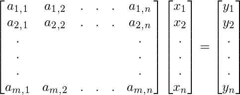+ a_m_, _n x_n = y_m$ which can also be written in matrix form as below: $\begin{bmatrix} a_1_, _1 & a_1_, _2&.&.&.&a_1_, _n \\ a_2_, _1 & a_2_, _2 &.&.&.&a_2_, _n\\ . & & & & & . \\ . & & & & & . \\ . & & & & & . \\ a_m_, _1 & a_m_, _2 &.&.&.&a_m_, _n\\ \end{bmatrix} % \begin{bmatrix} x_1\\ x_2\\ .\\ .\\ .\\ x_n\\ \end{bmatrix} = \begin{bmatrix} y_1\\ y_2\\ .\\ .\\ .\\ y_n\\ \end{bmatrix}$ Where m > n which means the number of rows is greater than the number of columns or the number of rows is greater than the number of variables. Solution to the above problem: There are multiple ways to solve the above problem. One solution involves Moore – Penrose Pseudoinverse. We write the Moore – Penrose pseudoinverse as $A^[+}$ . We have $A^{+}A = I$ but $AA^{+} \neq I$ unless A has the usual inverse. So, to solve the problem we proceed as follow: $\overrightarrow{y} = A\overrightarrow{x}$ $A^{+}\overrightarrow{y} \approx A^{+}A\overrightarrow{x}$ $A^{+}\overrightarrow{y} \approx I\overrightarrow{x}$ $A^{+}\overrightarrow{y} \approx \overrightarrow{x}$ This is how simply we solve the linear equations using the Moore – Penrose pseudoinverse. The derivation for Moore – Penrose pseudoinverse is beyond the scope of this article. You can go through this link in case you want to know more about it. Here, it is simply presented the method for computing it. The Moore – Penrose pseudoinverse is computed as $A^{+} = (A^{T} A)^{-1} A^{T}$ Example:

Consider below 3 linear equations:






Equivalently we can write above equations in matrix form as shown below:





After we compute the Moore - Penrose pseudoinverse using , we will get:



Check the matrix product  you will get identity matrix I.


We have,


Then,





After you compute above computation, you will get the final answer as

Note: Moore – Penrose pseudoinverse solves the problem in least squared error sense. In general, there is no exact solution to overdetermined problems. So if you cross check the solution you will not get the exact required y but an approx value of y.

Suggest improvement

Introduction to Speech Separation Based On Fast ICA

Sklearn | Feature Extraction with TF-IDF

Share your thoughts in the comments

Moore – Penrose Pseudoinverse | Mathematics

Please Login to comment...

Similar Reads

What kind of Experience do you want to share?