Monte Carlo integration in Python

Monte Carlo Integration is a process of solving integrals having numerous values to integrate upon. The Monte Carlo process uses the theory of large numbers and random sampling to approximate values that are very close to the actual solution of the integral. It works on the average of a function denoted by <f(x)>.  Then we can expand <f(x)> as the summation of the values divided by the number of points in the integration and solve the Left-hand side of the equation to approximate the value of the integration at the right-hand side. The derivation is as follows.

Where N = no. of terms used for approximation of the values.

Now we would first compute the integral using the Monte Carlo method numerically and then finally we would visualize the result using a histogram by using the python library matplotlib.

Modules Used:

The modules that would be used are:

• Scipy: Used to get random values between the limits of the integral. Can be installed using:

pip install scipy # for windows
or
pip3 install scipy # for linux and macos

• Numpy: Used to form arrays and store different values. Can be installed using:

pip install numpy # for windows
or 
pip3 install numpy # for linux and macos

• Matplotlib: Used to visualize the histogram and the result of the Monte Carlo integration.

pip install matplotlib # for windows
or 
pip3 install matplotlib # for linux and macos

Example 1:

The integral we are going to evaluate is:

Once we are done installing the modules, we can now start writing code by importing the required modules, scipy for creating random values in a range and NumPy module to create static arrays as default lists in python are relatively slow because of dynamic memory allocation. Then we defined the limits of integration which are 0 and pi (we used np.pi to get the value of pi. Then w create a static numpy array of zeros of size N using the np. zeros(N). Now we iterate over each index of array N and fill it with random values between a and b. Then we create a variable to store sum of the functions of different values of the integral variable. Now we create a function to calculate the sin of a particular value of x. Then we iterate and add up all the values returned by the function of x for different values of x to the variable integral. Then we use the formula derived above to get the results. Finally, we print the results on the final line.

Python3

# importing the modules
from scipy import random
import numpy as np

# limits of integration
a = 0
b = np.pi # gets the value of pi
N = 1000

# array of zeros of length N
ar = np.zeros(N)

# iterating over each Value of ar and filling
# it with a random value between the limits a
# and b
for i in range (len(ar)):
    ar[i] = random.uniform(a,b)

# variable to store sum of the functions of
# different values of x
integral = 0.0

# function to calculate the sin of a particular
# value of x
def f(x):
    return np.sin(x)

# iterates and sums up values of different functions
# of x
for i in ar:
    integral += f(i)

# we get the answer by the formula derived adobe
ans = (b-a)/float(N)*integral

# prints the solution
print ("The value calculated by monte carlo integration is {}.".format(ans))

Output:

The value calculated by monte carlo integration is 2.0256756150767035.

The value obtained is very close to the actual answer of the integral which is 2.0. 

Now if we want to visualize the integration using a histogram, we can do so by using the matplotlib library. Again we import the modules, define the limits of integration and write the sin function for calculating the sin value for a particular value of x. Next, we take an array that has variables representing every beam of the histogram. Then we iterate through N values and repeat the same process of creating a zeros array, filling it with random x values, creating an integral variable adding up all the function values, and getting the answer N times, each answer representing a beam of the histogram. The code is as follows:

Python3

# importing the modules
from scipy import random
import numpy as np
import matplotlib.pyplot as plt

# limits of integration
a = 0
b = np.pi # gets the value of pi
N = 1000

# function to calculate the sin of a particular
# value of x
def f(x):
    return np.sin(x)

# list to store all the values for plotting
plt_vals = []

# we iterate through all the values to generate
# multiple results and show whose intensity is
# the most.
for i in range(N):

    #array of zeros of length N
    ar = np.zeros(N)

    # iterating over each Value of ar and filling it
    # with a random value between the limits a and b
    for i in range (len(ar)):
        ar[i] = random.uniform(a,b)

    # variable to store sum of the functions of different
    # values of x
    integral = 0.0

    # iterates and sums up values of different functions
    # of x
    for i in ar:
        integral += f(i)

    # we get the answer by the formula derived adobe
    ans = (b-a)/float(N)*integral

    # appends the solution to a list for plotting the graph
    plt_vals.append(ans)

# details of the plot to be generated
# sets the title of the plot
plt.title("Distributions of areas calculated")

# 3 parameters (array on which histogram needs
plt.hist (plt_vals, bins=30, ec="black")

# to be made, bins, separators colour between the
# beams)
# sets the label of the x-axis of the plot
plt.xlabel("Areas")
plt.show() # shows the plot

Output:

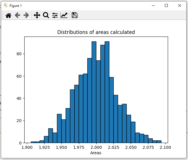
Here as we can see, the most probable results according to this graph would be 2.023 or 2.024 which is again quite close to the actual solution of this integral that is 2.0.  

Example 2:

The integral we are going to evaluate is: 

The implementation would be the same as the previous question, only the limits of integration defined by a and b would change and also the f(x) function that returns the corresponding function value of a specific value would now return x^2 instead of sin (x). The code for this would be: 

Python3

# importing the modules
from scipy import random
import numpy as np

# limits of integration
a = 0
b = 1
N = 1000

# array of zeros of length N
ar = np.zeros(N)

# iterating over each Value of ar and filling
# it with a random value between the limits a
# and b
for i in range(len(ar)):
    ar[i] = random.uniform(a, b)

# variable to store sum of the functions of
# different values of x
integral = 0.0

# function to calculate the sin of a particular
# value of x
def f(x):
    return x**2

# iterates and sums up values of different
# functions of x
for i in ar:
    integral += f(i)

# we get the answer by the formula derived adobe
ans = (b-a)/float(N)*integral

# prints the solution
print("The value calculated by monte carlo integration is {}.".format(ans))

Output:

The value calculated by monte carlo integration is 0.33024026610116575.

The value obtained is very close to the actual answer of the integral which is 0.333.

Now if we want to visualize the integration using a histogram again, we can do so by using the matplotlib library as we did for the previous expect in this case the f(x) functions return x^2 instead of sin(x), and the limits of integration change from 0 to 1.  The code is as follows:

Python3

# importing the modules
from scipy import random
import numpy as np
import matplotlib.pyplot as plt

# limits of integration
a = 0
b = 1
N = 1000

# function to calculate x^2 of a particular value
# of x
def f(x):
    return x**2

# list to store all the values for plotting
plt_vals = []

# we iterate through all the values to generate
# multiple results and show whose intensity is
# the most.
for i in range(N):

    # array of zeros of length N
    ar = np.zeros(N)

    # iterating over each Value of ar and filling
    # it with a random value between the limits a
    # and b
    for i in range (len(ar)):
        ar[i] = random.uniform(a,b)

    # variable to store sum of the functions of
    # different values of x
    integral = 0.0

    # iterates and sums up values of different functions
    # of x
    for i in ar:
        integral += f(i)

    # we get the answer by the formula derived adobe
    ans = (b-a)/float(N)*integral

    # appends the solution to a list for plotting the
    # graph
    plt_vals.append(ans)

# details of the plot to be generated
# sets the title of the plot
plt.title("Distributions of areas calculated")

# 3 parameters (array on which histogram needs
# to be made, bins, separators colour between
# the beams)
plt.hist (plt_vals, bins=30, ec="black")

# sets the label of the x-axis of the plot
plt.xlabel("Areas")
plt.show() # shows the plot

Output:

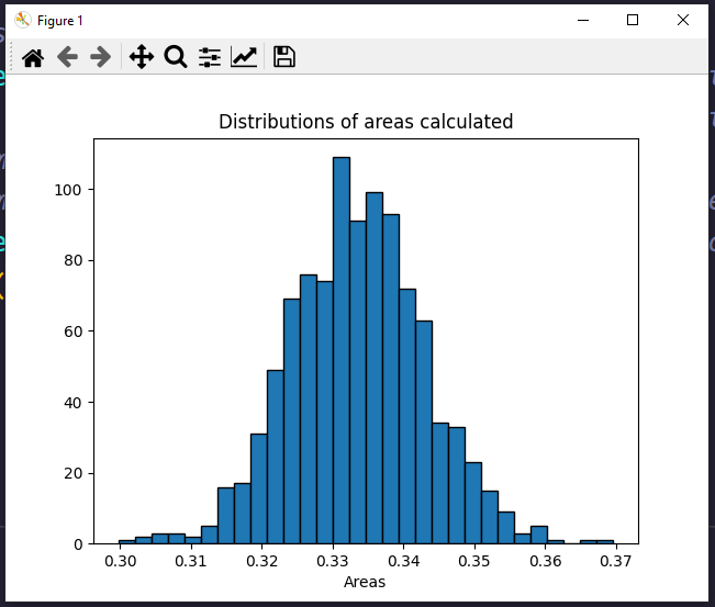
Here as we can see, the most probable results according to this graph would be 0.33 which is almost equal (equal in this case, but it generally doesn’t occur) to the actual solution of this integral that is 0.333.