MNIST Classification Using Multinomial Logistic + L1 in Scikit Learn

In this article, we shall implement MNIST classification using Multinomial Logistic Regression using the L1 penalty in the Scikit Learn Python library. 

Multinomial Logistic Regression and  L1 Penalty

MNIST is a widely used dataset for classification purposes. You may think of this dataset as the Hello World dataset of Machine Learning. Logistic Regression is a Supervised Machine Learning algorithm that is used in classification problem statements. Logistic Regression is also known as Binary(Binomial) Classification as it is mainly used to classify binary targets/labels as the predicted output. Whereas Multinomial Logistic regression is an extension of Logistic Regression which is used for Multi-class classification problems. 

Up next talking about the penalty in Logistic Regression we have L1 and L2 penalties. These penalties i.e., L1 and L2 are regularization methods used to reduce the overfitting effect. L1 penalty basically adds a sum of the absolute values of the parameters i.e, the sum of the weights. By adding this L1 penalty we push the features coefficients near 0. 

What is the L1 Penalty?

In Machine Learning, we have a specific terminology to define L1 and L2 regularization i.e., Lasso regression and Ridge Regression respectively. Here we will specifically cover Lasso Regression i.e., L1 penalty or regularization. 

The mathematically L1 penalty is defined as:

Lambda is a regularization constant, which plays a vital role in shrinking the weights. More the lambda value decreases the weights and results in a reduction in the cost function. Lasso regression aka L1 penalty is used to reduce the variance that helps in overfitting reduction. Using this method, we first sum up all the coefficients, if the coefficient terms increases, the above algorithm will penalize and shrink the value close to 0. 

MNIST Classification Using Multinomial Logistic + L1 in Scikit Learn

Now let’s start with importing the necessary libraries which we will be using to implement the multinomial logistic regression using the L1 penalty. Python libraries make it very easy for us to handle the data and perform typical and complex tasks with a single line of code.

• Pandas – This library helps to load the data frame in a 2D array format and has multiple functions to perform analysis tasks in one go.
• Numpy – Numpy arrays are very fast and can perform large computations in a very short time.
• Matplotlib/Seaborn – This library is used to draw visualizations.
• Sklearn – This module contains multiple libraries having pre-implemented functions to perform tasks from data preprocessing to model development and evaluation.

Python3

import pandas as pd
import matplotlib.pyplot as plt
from sklearn.linear_model import LogisticRegression
from sklearn.metrics import classification_report
from sklearn.model_selection import train_test_split

Load the Dataset

As the title suggests we will be using the MNIST Digit classification dataset in this article.

Python3

training = pd.read_csv('mnist/mnist_train.csv')
testing = pd.read_csv('mnist/mnist_test.csv')

print(training.shape)
print(testing.shape)

Output:

(60000, 785)
(10000, 785)

Python3

training.head()

Output:

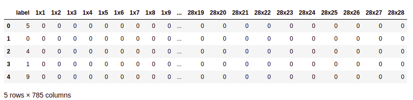
First five rows of the training data

Python3

testing.head()

Output:

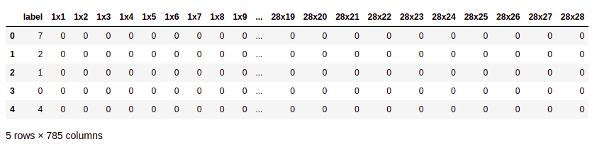
First five rows of the testing data

Data Visualization

Since MNIST is the Digit recognition dataset it consists of 70,000 images. In order to view these images, we need three dimension array. Each image is 28×28 pixels, by converting and reshaping the array we can visualize the dataset. 

Python3

X = training.drop('label', axis=1)
Y = training.label

plt.figure(figsize=(12, 10))
for img in range(1, 10):
    plt.subplot(3, 3, img)
    plt.imshow(X.loc[img].values.reshape(28, 28))
    plt.axis("off")

Output:

Some sample images from the datasets

Build Multinomial Logistic Regression and  L1  penalty model

To build a Multinomial Logistic Regression, we can assign multi_class=”multinomial”, but since the default value of multi_class=”auto” we do need to assign multi_class=”multinomial separately”. The auto will automatically assign the multinomial or binomial based on the unique target.

Talking about the other hyperparameter i.e., solver. For the Multinomial category, we assign the solver to be a saga. While dealing with L1 regularization, the saga is the most preferred solver. The reason has been, the Saga algorithm uses the SAG algorithm and applies an unbiased estimate of the full gradient with variance reduction constant α = 1. These SAG (Saga) algorithm performs well on sparse matrix, making them the best choice to be used for the Multinomial class category. 

The default penalty of Logistic Regression is l2, in our case, we can assign the penalty as l1. 

Python3

model = LogisticRegression(C=50.0, tol=0.01,
                           penalty="l1",
                           solver="saga")

model.fit(X, Y)

Model Evaluation

Now let’s check the performance of the trained model using the training data and the validation/testing data in this way we will be able to evaluate the model on completely new data as well as with the data on which it has been trained.

Python3

pred = model.predict(X)
print(classification_report(pred, Y))

Output:

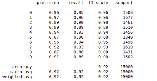
Classification report of the model on training data