ML | Normal Equation in Linear Regression
Last Updated :
10 Jun, 2023
We know the Linear Regression model is a parameterized model which means that the model’s behavior and predictions are determined by a set of parameters or coefficients in the model. However, we use different methods for finding these parameters which give the lowest error on our dataset. In this article, we will read one such article which is the normal equation.
Normal Equation
Normal Equation is an analytical approach to Linear Regression with a Least Square Cost Function. We can use the normal equation to directly compute the parameters of a model that minimizes the Sum of the squared difference between the actual term and the predicted term. This method is quite useful when the dataset is small. However, with a large dataset, it may not be able to give us the best parameter of the model.
The normal Equation is as follows:
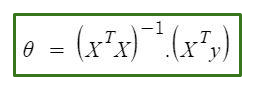
Normal equation formula
In the above equation,
θ: hypothesis parameters that define it the best.
X: Input feature value of each instance.
Y: Output value of each instance.
Maths Behind the Equation:
Given the hypothesis function

where,
n: the no. of features in the data set.
x0: 1 (for vector multiplication)
Notice that this is a dot product between θ and x values. So for the convenience to solve we can write it as:

The motive in Linear Regression is to minimize the cost function:
![J(\Theta) = \frac{1}{2m} \sum_{i = 1}^{m} \frac{1}{2} [h_{\Theta}(x^{(i)}) - y^{(i)}]^{2}](https://www.geeksforgeeks.org/wp-content/ql-cache/quicklatex.com-964ab765d209f44bdaf2dd3c4a8ed6a7_l3.png "Rendered by QuickLaTeX.com")
where,
xi: the input value of iih training example.
m: no. of training instances
n: no. of data-set features
yi: the expected result of ith instance
Let us represent the cost function in a vector form.
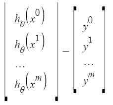
We have ignored 1/2m here as it will not make any difference in the working. It was used for mathematical convenience while calculating gradient descent. But it is no more needed here.
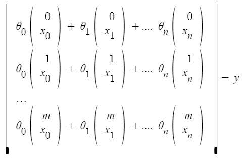
xij: the value of jih feature in iih training example.
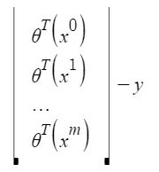
This can further be reduced to

But each residual value is squared. We cannot simply square the above expression. As the square of a vector/matrix is not equal to the square of each of its values. So to get the squared value, multiply the vector/matrix with its transpose. So, the final equation derived is

Therefore, the cost function is

Calculating the value of θ using the partial derivative of the Normal Equation
We will take a partial derivative of the cost function with respect to the parameter theta. Note that in partial derivative we treat all variables except the parameter theta as constant.


We know to find the optimum value of any partial derivative equation we have to equate it to 0.


Finally, we can solve for θ by multiplying both sides of the equation by the inverse of (2XᵀX):

We can implement this normal equation using Python programming language.
Python implementation of Normal Equation
We will create a synthetic dataset using sklearn having only one feature. Also, we will use numpy for mathematical computation like for getting the matrix to transform and inverse of the dataset. Also, we will use try and except block in our function so that in case if our input data matrix is singular our function will not be throwing an error.
Python3
import numpy as np
from sklearn.datasets import make_regression
X, y = make_regression(n_samples=100, n_features=1,
n_informative=1, noise=10, random_state=10)
def linear_regression_normal_equation(X, y):
X_transpose = np.transpose(X)
X_transpose_X = np.dot(X_transpose, X)
X_transpose_y = np.dot(X_transpose, y)
try:
theta = np.linalg.solve(X_transpose_X, X_transpose_y)
return theta
except np.linalg.LinAlgError:
return None
X_with_intercept = np.c_[np.ones((X.shape[0], 1)), X]
theta = linear_regression_normal_equation(X_with_intercept, y)
if theta is not None:
print(theta)
else:
print("Unable to compute theta. The matrix X_transpose_X is singular.")
|
Output:
[ 0.52804151 30.65896337]
To Predict on New Test Data Instances
Since we have trained our model and have found parameters that give us the lowest error. We can use this parameter to predict on new unseen test data.
Python3
def predict(X, theta):
predictions = np.dot(X, theta)
return predictions
X_test = np.array([[1], [4]])
X_test_with_intercept = np.c_[np.ones((X_test.shape[0], 1)), X_test]
predictions = predict(X_test_with_intercept, theta)
print("Predictions:", predictions)
|
Output:
Predictions: [ 31.18700488 123.16389501]
Like Article
Suggest improvement
Share your thoughts in the comments
Please Login to comment...