ML | Multiple Linear Regression using Python

Linear Regression:

It is the basic and commonly used type for predictive analysis. It is a statistical approach to modeling the relationship between a dependent variable and a given set of independent variables.

These are of two types:

1. Simple linear Regression
2. Multiple Linear Regression

Let’s Discuss Multiple Linear Regression using Python.

Multiple Linear Regression attempts to model the relationship between two or more features and a response by fitting a linear equation to observed data. The steps to perform multiple linear Regression are almost similar to that of simple linear Regression. The Difference Lies in the evaluation. We can use it to find out which factor has the highest impact on the predicted output and how different variables relate to each other.

Here : Y = b0 + b1 * x1 + b2 * x2 + b3 * x3 + …… bn * xn 
Y = Dependent variable and x1, x2, x3, …… xn = multiple independent variables 

Assumption of Regression Model : 

• Linearity: The relationship between dependent and independent variables should be linear.
• Homoscedasticity: Constant variance of the errors should be maintained.
• Multivariate normality: Multiple Regression assumes that the residuals are normally distributed.
• Lack of Multicollinearity: It is assumed that there is little or no multicollinearity in the data.

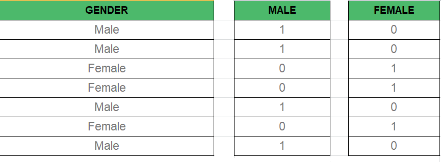
Dummy Variable:

As we know in the Multiple Regression Model we use a lot of categorical data. Using Categorical Data is a good method to include non-numeric data into the respective Regression Model. Categorical Data refers to data values that represent categories-data values with the fixed and unordered number of values, for instance, gender(male/female). In the regression model, these values can be represented by Dummy Variables. 
These variables consist of values such as 0 or 1 representing the presence and absence of categorical values. 

Dummy Variable Trap:
The Dummy Variable Trap is a condition in which two or more are Highly Correlated. In the simple term, we can say that one variable can be predicted from the prediction of the other. The solution of the Dummy Variable Trap is to drop one of the categorical variables. So if there are m Dummy variables then m-1 variables are used in the model. 

 D2 = D1-1   
 Here D2, D1 = Dummy Variables

Method of Building Models : 

• All-in
• Backward-Elimination
• Forward Selection
• Bidirectional Elimination
• Score Comparison

Backward-Elimination :

Step #1: Select a significant level to start in the model. 
Step #2: Fit the full model with all possible predictors. 
Step #3: Consider the predictor with the highest P-value. If P > SL go to STEP 4, otherwise the model is Ready. 
Step #4: Remove the predictor. 
Step #5: Fit the model without this variable.

Forward-Selection :

Step #1 : Select a significance level to enter the model(e.g. SL = 0.05) 
Step #2: Fit all simple regression models y~ x(n). Select the one with the lowest P-value. 
Step #3: Keep this variable and fit all possible models with one extra predictor added to the one(s) you already have. 
Step #4: Consider the predictor with the lowest P-value. If P < SL, go to Step #3, otherwise the model is Ready.

Steps Involved in any Multiple Linear Regression Model

Step #1: Data Pre Processing 

1. Importing The Libraries.
2. Importing the Data Set.
3. Encoding the Categorical Data.
4. Avoiding the Dummy Variable Trap.
5. Splitting the Data set into Training Set and Test Set.

Step #2: Fitting Multiple Linear Regression to the Training set 
Step #3: Predict the Test set results.

Code 1 : 

Python3

import numpy as np
import matplotlib as mpl
from mpl_toolkits.mplot3d import Axes3D
import matplotlib.pyplot as plt

def generate_dataset(n):
    x = []
    y = []
    random_x1 = np.random.rand()
    random_x2 = np.random.rand()
    for i in range(n):
        x1 = i
        x2 = i/2 + np.random.rand()*n
        x.append([1, x1, x2])
        y.append(random_x1 * x1 + random_x2 * x2 + 1)
    return np.array(x), np.array(y)

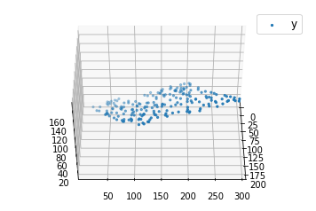
x, y = generate_dataset(200)

mpl.rcParams['legend.fontsize'] = 12

fig = plt.figure()
ax = fig.add_subplot(projection ='3d')

ax.scatter(x[:, 1], x[:, 2], y, label ='y', s = 5)
ax.legend()
ax.view_init(45, 0)

plt.show()

Output:

Code 2: 

Python3

def mse(coef, x, y):
    return np.mean((np.dot(x, coef) - y)**2)/2


def gradients(coef, x, y):
    return np.mean(x.transpose()*(np.dot(x, coef) - y), axis=1)


def multilinear_regression(coef, x, y, lr, b1=0.9, b2=0.999, epsilon=1e-8):
    prev_error = 0
    m_coef = np.zeros(coef.shape)
    v_coef = np.zeros(coef.shape)
    moment_m_coef = np.zeros(coef.shape)
    moment_v_coef = np.zeros(coef.shape)
    t = 0

    while True:
        error = mse(coef, x, y)
        if abs(error - prev_error) <= epsilon:
            break
        prev_error = error
        grad = gradients(coef, x, y)
        t += 1
        m_coef = b1 * m_coef + (1-b1)*grad
        v_coef = b2 * v_coef + (1-b2)*grad**2
        moment_m_coef = m_coef / (1-b1**t)
        moment_v_coef = v_coef / (1-b2**t)

        delta = ((lr / moment_v_coef**0.5 + 1e-8) *
                 (b1 * moment_m_coef + (1-b1)*grad/(1-b1**t)))

        coef = np.subtract(coef, delta)
    return coef


coef = np.array([0, 0, 0])
c = multilinear_regression(coef, x, y, 1e-1)
fig = plt.figure()
ax = fig.add_subplot(projection='3d')

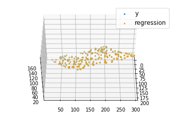
ax.scatter(x[:, 1], x[:, 2], y, label='y',
           s=5, color="dodgerblue")

ax.scatter(x[:, 1], x[:, 2], c[0] + c[1]*x[:, 1] + c[2]*x[:, 2],
           label='regression', s=5, color="orange")

ax.view_init(45, 0)
ax.legend()
plt.show()

Output:

Multiple linear regression is a statistical method used to model the relationship between multiple independent variables and a single dependent variable. In Python, the scikit-learn library provides a convenient implementation of multiple linear regression through the LinearRegression class.

Here’s an example of how to use LinearRegression to fit a multiple linear regression model in Python:

Python3

from sklearn.linear_model import LinearRegression
import numpy as np

# Assume you have independent variables X and a dependent variable y
X = np.array([[1, 2, 3], [2, 3, 4], [3, 4, 5], [4, 5, 6]])
y = np.array([1, 2, 3, 4])

# Create an instance of the LinearRegression class
reg = LinearRegression()

# Fit the model to the data
reg.fit(X, y)

# Print the coefficients of the model
print(reg.coef_)

This will output the coefficients of the multiple linear regression model, which can be used to make predictions about the dependent variable given new independent variable values.

It is important to mention that Linear Regression model should be used under certain assumption, such as Linearity, Homoscedasticity, Independence of errors, Normality of errors, and no multicollinearity, if these assumptions are not met, you should consider using other techniques or transforming your data.