Logistic Regression using Python
Last Updated :
04 Dec, 2023
A basic machine learning approach that is frequently used for binary classification tasks is called logistic regression. Though its name suggests otherwise, it uses the sigmoid function to simulate the likelihood of an instance falling into a specific class, producing values between 0 and 1. Logistic regression, with its emphasis on interpretability, simplicity, and efficient computation, is widely applied in a variety of fields, such as marketing, finance, and healthcare, and it offers insightful forecasts and useful information for decision-making.
Logistic Regression
A statistical model for binary classification is called logistic regression. Using the sigmoid function, it forecasts the likelihood that an instance will belong to a particular class, guaranteeing results between 0 and 1. To minimize the log loss, the model computes a linear combination of input characteristics, transforms it using the sigmoid, and then optimizes its coefficients using methods like gradient descent. These coefficients establish the decision boundary that divides the classes. Because of its ease of use, interpretability, and versatility across multiple domains, Logistic Regression is widely used in machine learning for problems that involve binary outcomes. Overfitting can be avoided by implementing regularization.
How the Logistic Regression Algorithm Works
Logistic Regression models the likelihood that an instance will belong to a particular class. It uses a linear equation to combine the input information and the sigmoid function to restrict predictions between 0 and 1. Gradient descent and other techniques are used to optimize the model’s coefficients to minimize the log loss. These coefficients produce the resulting decision boundary, which divides instances into two classes. When it comes to binary classification, logistic regression is the best choice because it is easy to understand, straightforward, and useful in a variety of settings. Generalization can be improved by using regularization.
Key Concepts of Logistic Regression
Important key concepts in logistic regression include:
- Sigmoid Function: The main function that ensures outputs are between 0 and 1 by converting a linear combination of input data into probabilities.
The sigmoid function is denoted as  , and is defined as:

Where, z is linear combination of input features and coefficients. - Hypothesis Function: uses the sigmoid function and weights (coefficients) to combine input features to estimate the likelihood of falling into a particular class.
In logistic regression, the hypothesis function is provided by:

Where,  is the predicted probability that y = 1,
  is the vector of coefficients, and x is the vector of input features.
 - Log Loss: The optimization cost function is a measure of the discrepancy between actual class labels and projected probability.
The definition of the log loss for a single instance is:

- Decision Boundary: The surface or line used to divide instances into several classes according to the determined probability.
- Probability Threshold: a number (usually 0.5) that is used to calculate the class assignment using the probabilities that are anticipated.
- Odds Ratio: The likelihood that an event will occur as opposed to not, which sheds light on how characteristics and the target variable are related.
Prerequisite: Understanding Logistic Regression
Implementation of Logistic Regression using Python
Import Libraries
Python3
import numpy as np
import pandas as pd
import matplotlib.pyplot as plt
import seaborn as sns
from sklearn.datasets import load_diabetes
from sklearn.model_selection import train_test_split
from sklearn.preprocessing import StandardScaler
from sklearn.linear_model import LogisticRegression
from sklearn.metrics import accuracy_score, classification_report, confusion_matrix, roc_curve, auc
|
Read and Explore the data
Python3
diabetes = load_diabetes()
X, y = diabetes.data, diabetes.target
y_binary = (y > np.median(y)).astype(int)
|
This code loads the diabetes dataset using the load_diabetes function from scikit-learn, passing in feature data X and target values y. Then, it converts the binary representation of the continuous target variable y. A patient’s diabetes measure is classified as 1 (indicating diabetes) if it is higher than the median value, and as 0 (showing no diabetes).
Splitting The Dataset: Train and Test dataset
Splitting the dataset to train and test. 80% of data is used for training the model and 20% of it is used to test the performance of our model.
Python3
X_train, X_test, y_train, y_test = train_test_split(
X, y_binary, test_size=0.2, random_state=42)
|
This code divides the diabetes dataset into training and testing sets using the train_test_split function from scikit-learn: The binary target variable is called y_binary, and the characteristics are contained in X. The data is divided into testing (X_test, y_test) and training (X_train, y_train) sets. Twenty percent of the data will be used for testing, according to the setting test_size=0.2. By employing a fixed seed for randomization throughout the split, random_state=42 guarantees reproducibility.
Feature Scaling
Python3
scaler = StandardScaler()
X_train = scaler.fit_transform(X_train)
X_test = scaler.transform(X_test)
|
This code uses StandardScaler from scikit-learn to achieve feature standardization:
The StandardScaler instance is created; this will be used to standardize the features. It uses the scaler’s fit_transform method to normalize the training data (X_train) and determine its mean and standard deviation. Then, itstandardizes the testing data (X_test) using the calculated mean and standard deviation from the training set. Model training and evaluation are made easier by standardization, which guarantees that the features have a mean of 0 and a standard deviation of 1.
Train The Model
Python3
model = LogisticRegression()
model.fit(X_train, y_train)
|
Using scikit-learn’s LogisticRegression, this code trains a logistic regression model:
It establishes a logistic regression model instance.Then, itemploys the fit approach to train the model using the binary target values (y_train) and standardized training data (X_train). Following execution, the model object may now be used to forecast new data using the patterns it has learnt from the training set.
Evaluation Metrics
Metrics are used to check the model performance on predicted values and actual values.
Python3
y_pred = model.predict(X_test)
accuracy = accuracy_score(y_test, y_pred)
print("Accuracy: {:.2f}%".format(accuracy * 100))
|
Output:
Accuracy: 73.03%
This code predicts the target variable and computes its accuracy in order to assess the logistic regression model on the test set. The accuracy_score function is then used to compare the predicted values in the y_pred array with the actual target values (y_test).
Confusion Matrix and Classification Report
Python3
print("Confusion Matrix:\n", confusion_matrix(y_test, y_pred))
print("\nClassification Report:\n", classification_report(y_test, y_pred))
|
Output:
Confusion Matrix:
 [[36 13]
 [11 29]]

Classification Report:
               precision    recall  f1-score   support

           0       0.77      0.73      0.75        49
           1       0.69      0.72      0.71        40

    accuracy                           0.73        89
   macro avg       0.73      0.73      0.73        89
weighted avg       0.73      0.73      0.73        89
Visualizing the performance of our model.
Python3
plt.figure(figsize=(8, 6))
sns.scatterplot(x=X_test[:, 2], y=X_test[:, 8], hue=y_test, palette={
0: 'blue', 1: 'red'}, marker='o')
plt.xlabel("BMI")
plt.ylabel("Age")
plt.title("Logistic Regression Decision Boundary\nAccuracy: {:.2f}%".format(
accuracy * 100))
plt.legend(title="Diabetes", loc="upper right")
plt.show()
|
Output:
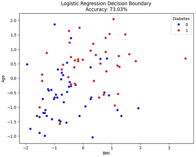
Logistic Regression
To see a logistic regression model’s decision border, this code creates a scatter plot. An individual from the test set is represented by each point on the plot, which has age on the Y-axis and BMI on the X-axis. The points are color-coded according to the actual status of diabetes, making it easier to evaluate how well the model differentiates between those with and without the disease. An instant visual context for the model’s performance on the test data is provided by the plot’s title, which includes the accuracy information. The inscription located in the upper right corner denotes the colors that represent diabetes (1) and no diabetes (0).
Plotting ROC Curve
Python3
y_prob = model.predict_proba(X_test)[:, 1]
fpr, tpr, thresholds = roc_curve(y_test, y_prob)
roc_auc = auc(fpr, tpr)
plt.figure(figsize=(8, 6))
plt.plot(fpr, tpr, color='darkorange', lw=2,
label=f'ROC Curve (AUC = {roc_auc:.2f})')
plt.plot([0, 1], [0, 1], color='navy', lw=2, linestyle='--', label='Random')
plt.xlabel('False Positive Rate')
plt.ylabel('True Positive Rate')
plt.title('Receiver Operating Characteristic (ROC) Curve\nAccuracy: {:.2f}%'.format(
accuracy * 100))
plt.legend(loc="lower right")
plt.show()
|
Output:

Receiver Operating Characteristic (ROC) Curve
For the logistic regression model, this code creates and presents the Receiver Operating Characteristic (ROC) curve. The true positive rate (sensitivity) and false positive rate at different threshold values are determined using the probability estimates for positive outcomes (y_prob), which are obtained using the predict_proba method. Use of the roc_auc_score yields the area under the ROC curve (AUC). An illustration of the resulting curve is provided, and the legend shows the AUC value. The ROC curve for a random classifier is shown by the dotted line.
Frequently Asked Questions
Q1. What is Logistic Regression?
A statistical technique for binary classification issues is called logistic regression.It uses a logistic function to model the likelihood of a binary outcome occurring.
Q2. How is Logistic Regression different from Linear Regression?
The probability of a binary event is predicted by logistic regression, whereas a continuous outcome is predicted by linear regression. In order to limit the output between 0 and 1, logistic regression uses the logistic (sigmoid) function.
Q3. How to handle categorical variables in Logistic Regression?
Use one-hot encoding, for instance, to transform categorical information into numerical representation. Make sure the data has been properly preprocessed to prepare it for logistic regression.
Q4. Can Logistic Regression handle multiclass classification?
It is possible to use methods like One-vs-Rest or Softmax Regression to expand logistic regression for multiclass classification.
Q5. What is the role of the sigmoid function in Logistic Regression?
Any real integer can be mapped to the range [0, 1] using the sigmoid function. The linear equation’s output is converted into probabilities by it.
Like Article
Suggest improvement
Share your thoughts in the comments
Please Login to comment...