ML | Introduction to Kernel PCA

PRINCIPAL COMPONENT ANALYSIS: is a tool which is used to reduce the dimension of the data. It allows us to reduce the dimension of the data without much loss of information. PCA reduces the dimension by finding a few orthogonal linear combinations (principal components) of the original variables with the largest variance. The first principal component captures most of the variance in the data. The second principal component is orthogonal to the first principal component and captures the remaining variance, which is left of first principal component and so on. There are as many principal components as the number of original variables. These principal components are uncorrelated and are ordered in such a way that the first several principal components explain most of the variance of the original data. To learn more about PCA you can read the article Principal Component Analysis

KERNEL PCA: PCA is a linear method. That is it can only be applied to datasets which are linearly separable. It does an excellent job for datasets, which are linearly separable. But, if we use it to non-linear datasets, we might get a result which may not be the optimal dimensionality reduction. Kernel PCA uses a kernel function to project dataset into a higher dimensional feature space, where it is linearly separable. It is similar to the idea of Support Vector Machines. There are various kernel methods like linear, polynomial, and gaussian. 

Kernel Principal Component Analysis (KPCA) is a technique used in machine learning for nonlinear dimensionality reduction. It is an extension of the classical Principal Component Analysis (PCA) algorithm, which is a linear method that identifies the most significant features or components of a dataset. KPCA applies a nonlinear mapping function to the data before applying PCA, allowing it to capture more complex and nonlinear relationships between the data points.

In KPCA, a kernel function is used to map the input data to a high-dimensional feature space, where the nonlinear relationships between the data points can be more easily captured by linear methods such as PCA. The principal components of the transformed data are then computed, which can be used for tasks such as data visualization, clustering, or classification.

One of the advantages of KPCA over traditional PCA is that it can handle nonlinear relationships between the input features, which can be useful for tasks such as image or speech recognition. KPCA can also handle high-dimensional datasets with many features by reducing the dimensionality of the data while preserving the most important information.

However, KPCA has some limitations, such as the need to choose an appropriate kernel function and its corresponding parameters, which can be difficult and time-consuming. KPCA can also be computationally expensive for large datasets, as it requires the computation of the kernel matrix for all pairs of data points.

References:

1. Schölkopf, B., Smola, A., & Müller, K. R. (1998). Nonlinear component analysis as a kernel eigenvalue problem. Neural computation, 10(5), 1299-1319.
2. Mika, S., Schölkopf, B., Smola, A. J., Müller, K. R., Scholz, M., & Rätsch, G. (1999). Kernel PCA and de-noising in feature spaces. Advances in neural information processing systems, 11, 536-542.
3. Shawe-Taylor, J., & Cristianini, N. (2004). Kernel methods for pattern analysis. Cambridge University Press.
   Overall, KPCA is a powerful tool for nonlinear dimensionality reduction and feature extraction, but it requires careful consideration of the choice of kernel
4. function and its parameters. It can be especially useful for high-dimensional datasets with complex relationships between the features.

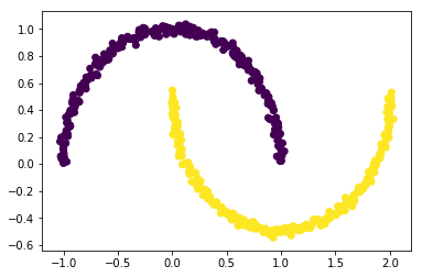
Code: Create a dataset that is nonlinear and then apply PCA to the dataset. 

Python3

import matplotlib.pyplot as plt
from sklearn.datasets import make_moons

X, y = make_moons(n_samples=500, noise=0.02, random_state=417)

plt.scatter(X[:, 0], X[:, 1], c=y)
plt.show()

Code: Let’s apply PCA to this dataset.

Python3

from sklearn.decomposition import PCA
pca = PCA(n_components=2)
X_pca = pca.fit_transform(X)

plt.title("PCA")
plt.scatter(X_pca[:, 0], X_pca[:, 1], c=y)
plt.xlabel("Component 1")
plt.ylabel("Component 2")
plt.show()

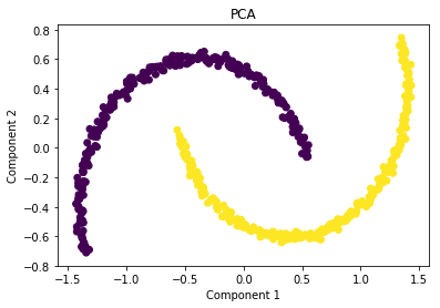
As you can see PCA failed to distinguish the two classes.   

Code: Applying kernel PCA on this dataset with RBF kernel with a gamma value of 15. 

Python3

from sklearn.decomposition import KernelPCA
kpca = KernelPCA(kernel='rbf', gamma=15)
X_kpca = kpca.fit_transform(X)

plt.title("Kernel PCA")
plt.scatter(X_kpca[:, 0], X_kpca[:, 1], c=y)
plt.show()

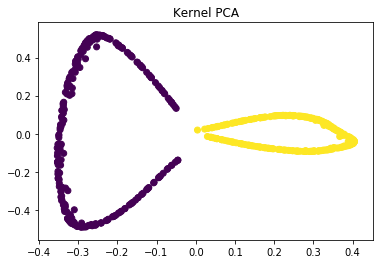
In the kernel space the two classes are linearly separable. Kernel PCA uses a kernel function to project the dataset into a higher-dimensional space, where it is linearly separable. Finally, we applied the kernel PCA to a non-linear dataset using scikit-learn. 

Kernel Principal Component Analysis (PCA) is a technique for dimensionality reduction in machine learning that uses the concept of kernel functions to transform the data into a high-dimensional feature space. In traditional PCA, the data is transformed into a lower-dimensional space by finding the principal components of the covariance matrix of the data. In kernel PCA, the data is transformed into a high-dimensional feature space using a non-linear mapping function, called a kernel function, and then the principal components are found in this high-dimensional space.

Advantages of Kernel PCA:

1. Non-linearity: Kernel PCA can capture non-linear patterns in the data that are not possible with traditional linear PCA.
2. Robustness: Kernel PCA can be more robust to outliers and noise in the data, as it considers the global structure of the data, rather than just local distances between data points.
3. Versatility: Different types of kernel functions can be used in kernel PCA to suit different types of data and different objectives.
4. Kernel PCA can handle nonlinear relationships between the input features, allowing for more accurate dimensionality reduction and feature extraction compared to traditional linear PCA.
5. It can preserve the most important information in high-dimensional datasets while reducing the dimensionality of the data, making it easier to visualize and analyze.
6. Kernel PCA can be used for a variety of tasks, including data visualization, clustering, and classification.
7. It is a well-established and widely used technique in machine learning, with many available libraries and resources for implementation.

Disadvantages of Kernel PCA:

1. Complexity: Kernel PCA can be computationally expensive, especially for large datasets, as it requires the calculation of eigenvectors and eigenvalues.
2. Model selection: Choosing the right kernel function and the right number of components can be challenging and may require expert knowledge or trial and error
3. Choosing an appropriate kernel function and its parameters can be challenging and may require expert knowledge or extensive experimentation.
4. Kernel PCA can be computationally expensive, especially for large datasets, as it requires the computation of the kernel matrix for all pairs of data points.
5. It may not always be easy to interpret the results of kernel PCA, as the transformed data may not have a clear interpretation in the original feature space.
6. Kernel PCA is not suitable for datasets with many missing values or outliers, as it assumes a complete and consistent dataset.