Frequent Pattern Growth Algorithm

Prerequisites: Apriori Algorithm ,Trie Data structure

The two primary drawbacks of the Apriori Algorithm are: 

1. At each step, candidate sets have to be built.
2. To build the candidate sets, the algorithm has to repeatedly scan the database.

These two properties inevitably make the algorithm slower. To overcome these redundant steps, a new association-rule mining algorithm was developed named Frequent Pattern Growth Algorithm. It overcomes the disadvantages of the Apriori algorithm by storing all the transactions in a Trie Data Structure. Consider the following data:- 

[Tex]\begin{array}{|c|c|} \hline \textbf{Transaction ID} & \textbf{Items} \\ \hline \mathrm{T} 1 & \{\mathrm{E}, \mathrm{K}, \mathrm{M}, \mathrm{N}, \mathrm{O}, \mathrm{Y}\} \\ \hline \mathrm{T} 2 & \{\mathrm{D}, \mathrm{E}, \mathrm{K}, \mathrm{N}, \mathbf{O}, \mathrm{Y}\} \\ \hline \mathrm{T} 3 & \{\mathrm{A}, \mathrm{E}, \mathrm{K}, \mathrm{M}\} \\ \hline \mathrm{T} 4 & \{\mathrm{C}, \mathrm{K}, \mathrm{M}, \mathrm{U}, \mathrm{Y}\} \\ \hline \mathrm{T} 5 & \{\mathrm{C}, \mathrm{E}, \mathrm{I}, \mathrm{K}, \mathrm{O}, \mathrm{O}\} \\ \hline \end{array}[/Tex]

The above-given data is a hypothetical dataset of transactions with each letter representing an item. The frequency of each individual item is computed:- 

[Tex]\begin{array}{|c|c|} \hline \textbf { Item } & \textbf { Frequency } \\ \hline \mathbf{A} & \mathbf{1} \\ \hline \mathbf{C} & \mathbf{2} \\ \hline \mathbf{D} & \mathbf{1} \\ \hline \mathbf{E} & \mathbf{4} \\ \hline \mathbf{I} & \mathbf{1} \\ \hline \mathbf{K} & \mathbf{5} \\ \hline \mathbf{M} & \mathbf{3} \\ \hline \mathbf{N} & \mathbf{2} \\ \hline \mathbf{O} & \mathbf{4} \\ \hline \mathbf{U} & \mathbf{1} \\ \hline \mathbf{Y} & \mathbf{3} \\ \hline \end{array}[/Tex]

Let the minimum support be 3. A Frequent Pattern set is built which will contain all the elements whose frequency is greater than or equal to the minimum support. These elements are stored in descending order of their respective frequencies. After insertion of the relevant items, the set L looks like this:- 

L = {K : 5, E : 4, M : 3, O : 4, Y : 3}

Now, for each transaction, the respective Ordered-Item set is built. It is done by iterating the Frequent Pattern set and checking if the current item is contained in the transaction in question. If the current item is contained, the item is inserted in the Ordered-Item set for the current transaction. The following table is built for all the transactions: 

[Tex]\begin{array}{|c|c|c|} \hline \textbf {Transaction ID} & \textbf {Items} & \textbf {Ordered-Item Set} \\ \hline \mathrm{T} 1 & \{\mathrm{E}, \mathrm{K}, \mathrm{M}, \mathrm{N}, \mathrm{O}, \mathrm{Y}\} & \{\mathrm{K}, \mathrm{E}, \mathrm{M}, \mathrm{O}, \mathrm{Y}\} \\ \hline \mathrm{T} 2 & \{\mathrm{D}, \mathrm{E}, \mathrm{K}, \mathrm{N}, \mathrm{O}, \mathrm{Y}\} & \{\mathrm{K}, \mathrm{E}, \mathrm{O}, \mathrm{Y}\} \\ \hline \mathrm{T} 3 & \{\mathrm{A}, \mathrm{E}, \mathrm{K},\mathrm{M}\} & \{\mathrm{K}, \mathrm{E}, \mathrm{M}\} \\ \hline \mathrm{T} 4 & \{\mathrm{C}, \mathrm{K}, \mathrm{M},\mathrm{U}, \mathrm{Y}\} & \{\mathrm{K}, \mathrm{M}, \mathrm{Y}\} \\ \hline \mathrm{T} 5 & \{\mathrm{C}, \mathrm{E}, \mathrm{I},\mathrm{K}, \mathrm{O}, \mathrm{O}\} & \{\mathrm{K}, \mathrm{E}, \mathrm{O}\} \\ \hline \end{array}[/Tex]

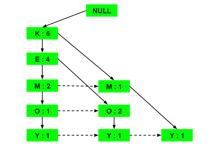
Now, all the Ordered-Item sets are inserted into a Trie Data Structure. 

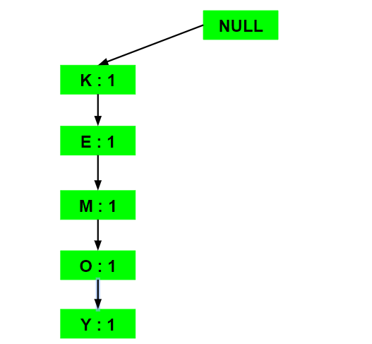
a) Inserting the set {K, E, M, O, Y}:

Here, all the items are simply linked one after the other in the order of occurrence in the set and initialize the support count for each item as 1. 

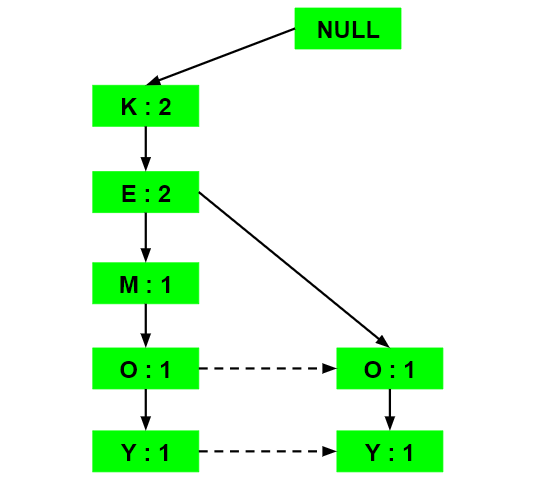
b) Inserting the set {K, E, O, Y}:

Till the insertion of the elements K and E, simply the support count is increased by 1. On inserting O we can see that there is no direct link between E and O, therefore a new node for the item O is initialized with the support count as 1 and item E is linked to this new node. On inserting Y, we first initialize a new node for the item Y with support count as 1 and link the new node of O with the new node of Y. 

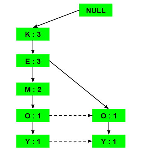
c) Inserting the set {K, E, M}:

Here simply the support count of each element is increased by 1. 

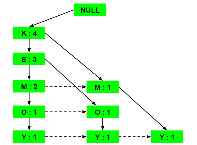
d) Inserting the set {K, M, Y}:

Similar to step b), first the support count of K is increased, then new nodes for M and Y are initialized and linked accordingly. 

e) Inserting the set {K, E, O}:

Here simply the support counts of the respective elements are increased. Note that the support count of the new node of item O is increased. 

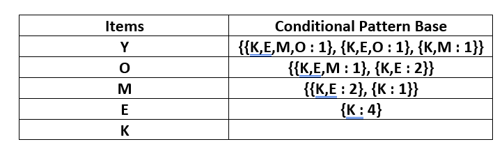
Now, for each item, the Conditional Pattern Base is computed which is path labels of all the paths which lead to any node of the given item in the frequent-pattern tree. Note that the items in the below table are arranged in the ascending order of their frequencies. 

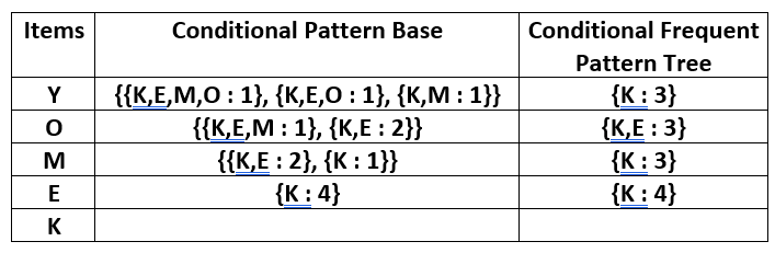
Now for each item, the Conditional Frequent Pattern Tree is built. It is done by taking the set of elements that is common in all the paths in the Conditional Pattern Base of that item and calculating its support count by summing the support counts of all the paths in the Conditional Pattern Base. 

From the Conditional Frequent Pattern tree, the Frequent Pattern rules are generated by pairing the items of the Conditional Frequent Pattern Tree set to the corresponding to the item as given in the below table. 

For each row, two types of association rules can be inferred for example for the first row which contains the element, the rules K -> Y and Y -> K can be inferred. To determine the valid rule, the confidence of both the rules is calculated and the one with confidence greater than or equal to the minimum confidence value is retained.