ML – Different Regression types
Last Updated :
22 Jul, 2021
Regression Analysis:
It is a form of predictive modelling technique which investigates the relationship between a dependent (target) and independent variable (s) (predictor).
To establish the possible relationship among different variables, various modes of statistical approaches are implemented, known as regression analysis. Basically, regression analysis sets up an equation to explain the significant relationship between one or more predictors and response variables and also to estimate current observations. Regression model comes under the supervised learning, where we are trying to predict results within a continuous output, meaning that we are trying to map input variables to some continuous function. Predicting prices of a house given the features of the house like size, price etc is one of the common examples of Regression
Types of regression in ML
- Linear Regression :
Linear regression attempts to model the relationship between two variables by fitting a linear equation to observed data. One variable is considered to be an explanatory variable, and the other is considered to be a dependent variable.It is represented by an equation:
Y = a + b*X + e
where a is intercept, b is slope of the line and e is error term. This equation can be used to predict the value of target variable based on given predictor variable(s).This can be written much more concisely using a vectorized form, as shown:
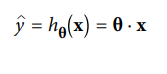
where h? is the hypothesis function, using the model parameters ?.
-
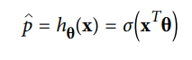
Logistic Regression: Some regression algorithm can also be used for classification.Logistic regression is commonly used to estimate the probability that an instance belongs to a particular class. For example, what is the probability that this email is spam?. If the estimated probability is greater than 50% then the instance belongs to that class called the positive class(1) or else it predicts that it does not then it belongs to the negative class(0). This makes it a binary classification.
In order to map predicted values to probabilities, we use the sigmoid function. The function maps any real value into another value between 0 and 1.
y = 1/(1 + e(-x)).
This linear relationship can be written in the following mathematical form:
-
Polynomial Regression: What if our data is actually more complex than a simple straight line? Surprisingly, we can actually use a linear model to fit nonlinear data. A simple way to do this is to add powers of each feature as new features, then train a linear model on this extended set of features. This technique is called Polynomial Regression.The equation below represents a polynomial equation:

-
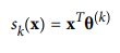
Softmax Regression: The Logistic Regression model can be generalized to support multiple classes directly, without having to train and combine multiple binary classifiers . This is called Somax Regression, or Multinomial Logistic Regression.The idea is quite simple: when given an instance x, the Softmax Regression model first computes a score sk(x) for each class k, then estimates the probability of each class by applying the somax function (also called the normalized exponential) to the scores.Equation for softmax regression:
-
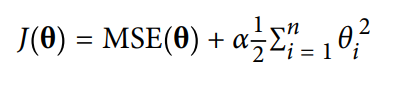
Ridge Regression: Rigid Regression is a regularized version of Linear Regression where a regularized term is added to the cost function. This forces the learning algorithm to not only fit the data but also keep the model weights as small as possible. Note that the regularized term should not be added to the cost function during training. Once the model is trained, you want to evaluate the model’s performance using the unregularized performance measure. The formula for rigid regression is:
-
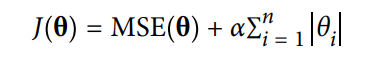
Lasso Regression: Similar to Ridge Regression, Lasso (Least Absolute Shrinkage and Selection Operator) is another regularized version of Linera regression : it adds a regularized term to the cost function, but it uses the l1 norm of the weighted vector instead of half the square of the l2 term Lasso regression is given as:
-
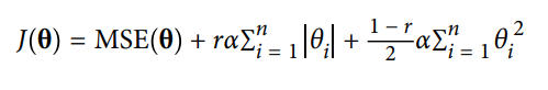
Elastic Net Regression: ElasticNet is middle ground between Lasso and Ridge Regression techniques.The regularization term is a simple mix of both Rigid and Lasso’s regularization term. when r=0, Elastic Net is equivalent to Rigid Regression and when r=1, Elastic Net is equivalent to Lasso Regression.The expression for Elastic Net Regression is given as:
Need for regression:
If we want to do any sort of data analysis on the given data, we need to establish a proper relationship between the dependent and independent variables to do predictions which forms the basis of our evaluation. And that relationships are given by the regression models and thus they form the core for any data analysis.
Gradient Descent:
Gradient Descent is a very generic optimization algorithm capable of finding optimal solutions to a wide range of problems. The general idea of Gradient Descent is to tweak parameters iteratively in order to minimize a cost function. Here that function is our Loss Function. The loss is the error in our predicted value of m(slope) and c(constant). Our goal is to minimize this error to obtain the most accurate value of m and c.
We will use the Mean Squared Error function to calculate the loss. There are three steps in this function:
- Find the difference between the actual y and predicted y value(y = mx + c), for a given x.
- Square this difference.
- Find the mean of the squares for every value in X.
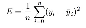
Here y is the actual value and y’ is the predicted value. Lets substitute the value of y’: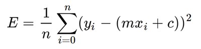
Now the above equation is minimized using the gradient descent algorithm by partially differentiating it w.r.t m and c.
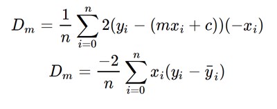
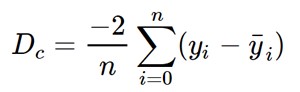
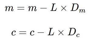
Then finally we update the values of m and c as follow:
Code: simple demonstration of Gradient Descent
import pandas as pd
import numpy as np
import matplotlib as mpl
import matplotlib.pyplot as plt
X = np.arange(1, 7)
Y = X**2
plt.figure(figsize =(10, 10))
plt.scatter(X, y, color ="yellow")
plt.title('sample demonstration of gradient descent')
plt.ylabel('squared value-y')
plt.xlabel('linear value-x')
|
Output:
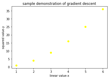
scatter plot
Code:
m = 0
c = 0
L = 0.0001
epochs = 1000
n = float(len(X))
for i in range(epochs):
Y_pred = m * X + c
D_m = (-2 / n) * sum(X * (Y - Y_pred))
D_c = (-2 / n) * sum(Y - Y_pred)
m = m - L * D_m
c = c - L * D_c
print (m, c)
|
Output:
4.471681318702568 0.6514172394787497
Code:
Y_pred = m * X + c
plt.figure(figsize =(10, 10))
plt.scatter(X, Y, color ="yellow")
plt.plot([min(X), max(X)], [min(Y_pred), max(Y_pred)], color ='red')
plt.title('sample demonstration of gradient descent')
plt.ylabel('squared value-y')
plt.xlabel('linear value-x')
plt.show()
|
Output:
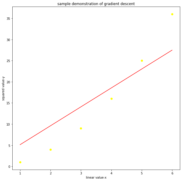
final result
Like Article
Suggest improvement
Share your thoughts in the comments
Please Login to comment...