ML | Common Loss Functions

The loss function estimates how well a particular algorithm models the provided data. Loss functions are classified into two classes based on the type of learning task

• Regression Models: predict continuous values.
• Classification Models: predict the output from a set of finite categorical values.

REGRESSION LOSSES

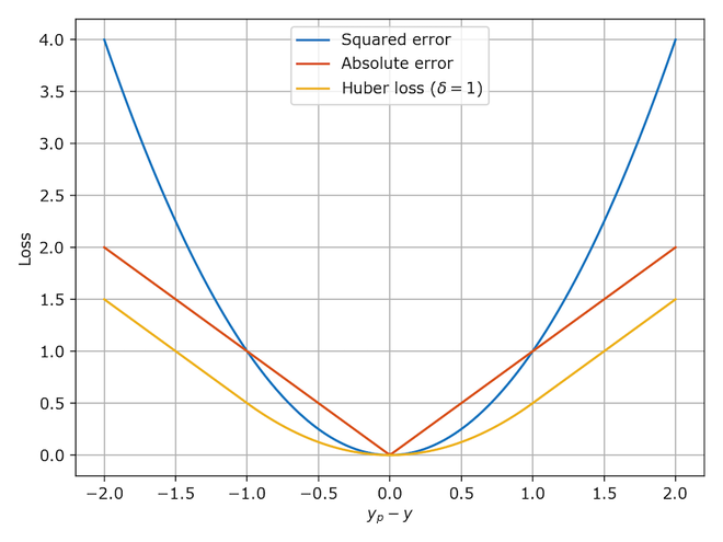
Mean Squared Error (MSE) / Quadratic Loss / L2 Loss

• It is the Mean of Square of Residuals for all the datapoints in the dataset. Residuals is the difference between the actual and the predicted prediction by the model.
• Squaring of residuals is done to convert negative values to positive values. The normal error can be both negative and positive. If some positive and negative numbers are summed up, the sum maybe 0. This will tell the model that the net error is 0 and the model is performing well but contrary to that, the model is still performing badly. Thus, to get the actual performance of the model, only positive values are taken to get positive, squaring is done.
• Squaring also gives more weightage to larger errors. When the cost function is far away from its minimal value, squaring the error will penalize the model more and thus helping in reaching the minimal value faster.
• Mean of the Square of Residuals is taking instead of just taking the sum of square of residuals to make the loss function independent of number of datapoints in the training set.
• MSE is sensitive to outliers. 

(1)

Python3

import numpy as np

# Mean Squared Error

def mse( y, y_pred ) :

    return  np.sum( ( y - y_pred ) ** 2 ) / np.size( y )

where,
i        - ith training sample in a dataset
n        - number of training samples
y(i)     - Actual output of ith training sample
y-hat(i) - Predicted value of ith training sample

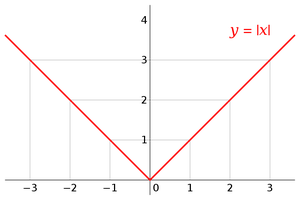
Mean Absolute Error (MAE) / La Loss

• It is the Mean of Absolute of Residuals for all the datapoints in the dataset. Residuals is the difference between the actual and the predicted prediction by the model.
• The absolute of residuals is done to convert negative values to positive values.
• Mean is taken to make the loss function independent of number of datapoints in the training set.
• One advantage of MAE is that is robust to outliers.
• MAE is generally less preferred over MSE as it is harder to calculate the derivative of the absolute function because absolute function is not differentiable at the minima.

Source: Wikipedia

(2)

Python3

# Mean Absolute Error

def mae( y, y_pred ) :

    return np.sum( np.abs( y - y_pred ) ) / np.size( y )

Output

Mean Bias Error: It is the same as MSE. but less accurate and can could conclude if the model has a positive bias or negative bias. 

(3)

Python3

# Mean Bias Error

def mbe( y, y_pred ) :

    return np.sum( y - y_pred ) / np.size( y )

Output

Huber Loss / Smooth Mean Absolute Error

• It is the combination of MSE and MAE. It takes the good properties of both the loss functions by being less sensitive to outliers and differentiable at minima.
• When the error is smaller, the MSE part of the Huber is utilized and when the error is large, the MAE part of Huber loss is used.
• A new hyper-parameter ‘????‘ is introduced which tells the loss function where to switch from MSE to MAE.
• Additional ‘????’ terms are introduced in the loss function to smoothen the transition from MSE to MAE. 

Source: www.evergreeninnovations.co

(4)

Python3

def Huber(y, y_pred, delta):

    condition = np.abs(y - y_pred) < delta

    l = np.where(condition, 0.5 * (y - y_pred) ** 2,
                 delta * (np.abs(y - y_pred) - 0.5 * delta))

    return np.sum(l) / np.size(y)

Output

CLASSIFICATION LOSSES

Cross-Entropy Loss: Also known as Negative Log Likelihood. It is the commonly used loss function for classification. Cross-entropy loss progress as the predicted probability diverges from the actual label.

Python3

# Binary Loss


def cross_entropy(y, y_pred):

    return - np.sum(y * np.log(y_pred) + (1 - y) * np.log(1 - y_pred)) / np.size(y)

Output

(5)

Hinge Loss:  Also known as Multi-class SVM Loss. Hinge loss is applied for maximum-margin classification, prominently for support vector machines. It is a convex function used in the convex optimizer. 

(6)

Python3

# Hinge Loss


def hinge(y, y_pred):

    l = 0

    size = np.size(y)

    for i in range(size):

        l = l + max(0, 1 - y[i] * y_pred[i])

    return l / size

Output