Microsoft Stock Price Prediction with Machine Learning

In this article, we will implement Microsoft Stock Price Prediction with a Machine Learning technique. We will use TensorFlow, an Open-Source Python Machine Learning Framework developed by Google. TensorFlow makes it easy to implement Time Series forecasting data. Since Stock Price Prediction is one of the Time Series Forecasting problems, we will build an end-to-end Microsoft Stock Price Prediction with a Machine learning technique. 

Importing Libraries and Dataset

Python libraries make it very easy for us to handle the data and perform typical and complex tasks with a single line of code.

• Pandas – This library helps to load the data frame in a 2D array format and has multiple functions to perform analysis tasks in one go.
• Numpy – Numpy arrays are very fast and can perform large computations in a very short time.
• Matplotlib/Seaborn – This library is used to draw visualizations.
• Sklearn – This module contains multiple libraries having pre-implemented functions to perform tasks from data preprocessing to model development and evaluation.
• Tensorflow – TensorFlow is a Machine Learning Framework developed by Google Developers to make the implementation of machine learning algorithms a cakewalk.

Python3

from datetime import datetime
import tensorflow as tf
from tensorflow import keras
import pandas as pd
import matplotlib.pyplot as plt
from sklearn.preprocessing import StandardScaler
import numpy as np
import seaborn as sns

Now let’s load the dataset which contains the OHLC data about the Microsoft Stock for the tradable days. You can download the dataset which has been used here.

Python3

microsoft = pd.read_csv('MicrosoftStock.csv')
print(microsoft.head())

Output:

         date   open   high    low  close    volume Name
0  2013-02-08  15.07  15.12  14.63  14.75   8407500  AAL
1  2013-02-11  14.89  15.01  14.26  14.46   8882000  AAL
2  2013-02-12  14.45  14.51  14.10  14.27   8126000  AAL
3  2013-02-13  14.30  14.94  14.25  14.66  10259500  AAL
4  2013-02-14  14.94  14.96  13.16  13.99  31879900  AAL

Python3

microsoft.shape

Output:

(619040, 7)

Python3

microsoft.info()

Output:

<class 'pandas.core.frame.DataFrame'>
RangeIndex: 619040 entries, 0 to 619039
Data columns (total 7 columns):
 #   Column  Non-Null Count   Dtype         
---  ------  --------------   -----         
 0   date    619040 non-null  datetime64[ns]
 1   open    619029 non-null  float64       
 2   high    619032 non-null  float64       
 3   low     619032 non-null  float64       
 4   close   619040 non-null  float64       
 5   volume  619040 non-null  int64         
 6   Name    619040 non-null  object        
dtypes: datetime64[ns](1), float64(4), int64(1), object(1)
memory usage: 33.1+ MB

Python3

microsoft.describe()

Output:

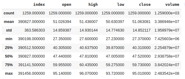
Descriptive statistical measures of the features.

Exploratory Data Analysis

EDA is an approach to analyzing the data using visual techniques. It is used to discover trends, and patterns, or to check assumptions with the help of statistical summaries and graphical representations. 

Python3

plt.plot(microsoft['date'],
         microsoft['open'],
         color="blue",
         label="open")
plt.plot(microsoft['date'],
         microsoft['close'],
         color="green",
         label="close")
plt.title("Microsoft Open-Close Stock")
plt.legend()

Output:

Trends in the prices of Microsoft Stock over the years

Python3

plt.plot(microsoft['date'],
         microsoft['volume'])
plt.show()

Output:

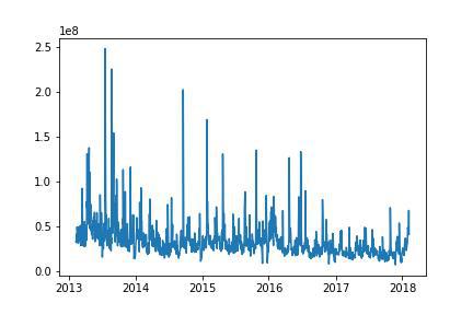
Trends in the volumes of trade of Microsoft Stock over the years

Python3

sns.heatmap(microsoft.corr(),
            annot=True,
            cbar=False)
plt.show()

Output:

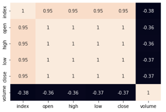
Heatmap too analyzes the correlation between different features

Now, let’s just plot the Close prices of Microsoft Stock for the time period of 2013 to 2018 which is for a span of 5 years.

Python3

microsoft['date'] = pd.to_datetime(microsoft['date'])
prediction = microsoft.loc[(microsoft['date']
                            > datetime(2013, 1, 1))
                            & (microsoft['date']
                            < datetime(2018, 1, 1))]

plt.figure(figsize=(10, 10))
plt.plot(microsoft['date'], microsoft['close'])
plt.xlabel("Date")
plt.ylabel("Close")
plt.title("Microsoft Stock Prices")

Output:

Trends in the Close price of trade of Microsoft Stock over the years

Python3

# prepare the training set samples
msft_close = microsoft.filter(['close'])
dataset = msft_close.values
training = int(np.ceil(len(dataset) *. 95))

# scale the data
ss = StandardScaler()
ss = ss.fit_transform(dataset)

train_data = ss[0:int(training), :]

x_train = []
y_train = []

# considering 60 as the batch size,
# create the X_train and y_train
for i in range(60, len(train_data)):
    x_train.append(train_data[i-60:i, 0])
    y_train.append(train_data[i, 0])

x_train, y_train = np.array(x_train),\
                   np.array(y_train)
X_train = np.reshape(x_train,
                     (x_train.shape[0],
                      x_train.shape[1], 1))

Build the Model

To tackle the Time Series or Stock Price Prediction problem statement, we build a Recurrent Neural Network model, that comes in very handy to memorize the previous state using cell state and memory state. Since RNNs are hard to train and prune to Vanishing Gradient, we use LSTM which is the RNN gated cell, LSTM reduces the problem of Vanishing gradients. 

Python3

model = keras.models.Sequential()
model.add(keras.layers.LSTM(units=64,
                            return_sequences=True,
                            input_shape
                            =(X_train.shape[1], 1)))
model.add(keras.layers.LSTM(units=64))
model.add(keras.layers.Dense(128))
model.add(keras.layers.Dropout(0.5))
model.add(keras.layers.Dense(1))

print(model.summary())

Output:

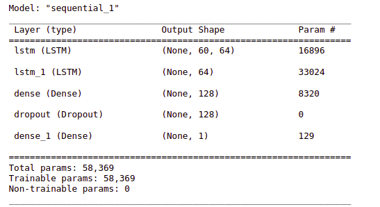
Summary of the architecture of the model

Compile and Fit

While compiling a model we provide these three essential parameters:

• optimizer – This is the method that helps to optimize the cost function by using gradient descent.
• loss – The loss function by which we monitor whether the model is improving with training or not.
• metrics – This helps to evaluate the model by predicting the training and the validation data.

Python3

from keras.metrics import RootMeanSquaredError
model.compile(optimizer='adam',
              loss='mae',
              metrics=RootMeanSquaredError())

history = model.fit(X_train, y_train,
                    epochs=20)

Output:

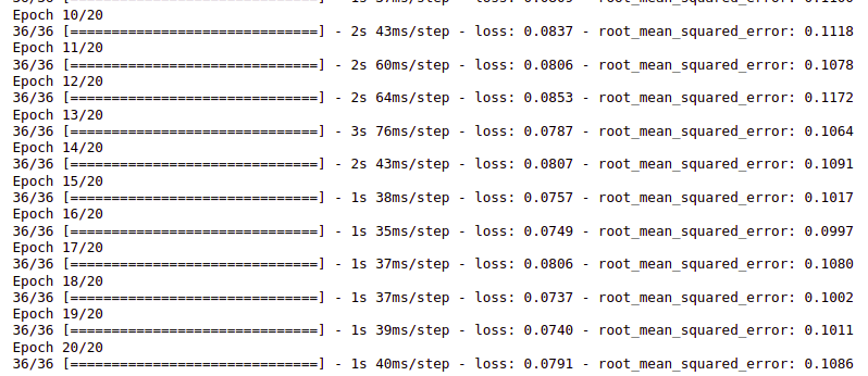
Training progress of the LSTM model

We got 0.0791 mean absolute error, which is close to the perfect error score. 

Model Evaluation

Now as we have our model ready let’s evaluate its performance on the validation data using different metrics. For this purpose, we will first predict the class for the validation data using this model and then compare the output with the true labels.

Python3

testing = ss[training - 60:, :]
x_test = []
y_test = dataset[training:, :]
for i in range(60, len(testing)):
    x_test.append(testing[i-60:i, 0])

x_test = np.array(x_test)
X_test = np.reshape(x_test,
                    (x_test.shape[0],
                     x_test.shape[1], 1))

pred = model.predict(X_test)

Output:

2/2 [==============================] - 2s 35ms/step

Now let’s plot the known data and the predicted price trends in the Microsoft Stock prices and see whether they align with the previous trends or totally different from them.

Python3

train = microsoft[:training]
test = microsoft[training:]
test['Predictions'] = pred

plt.figure(figsize=(10, 8))
plt.plot(train['close'], c="b")
plt.plot(test[['close', 'Predictions']])
plt.title('Microsoft Stock Close Price')
plt.ylabel("Close")
plt.legend(['Train', 'Test', 'Predictions'])

Output:

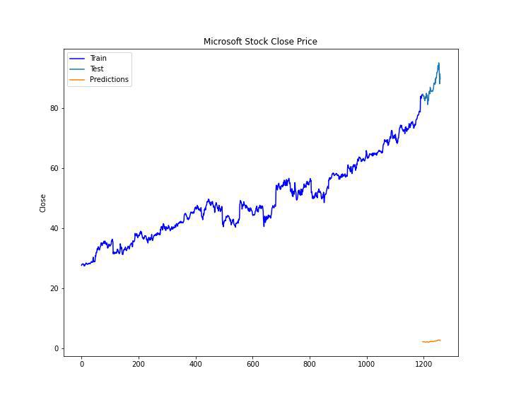
Predicted and the known stock prices