Mean, Median and Mode of Grouped Data

Suppose we want to compare the age of students in two schools and determine which school has more aged students. If we compare on the basis of individual students, we cannot conclude anything. However, if for the given data, we get a representative value that signifies the characteristics of the data, the comparison becomes easy. 

A certain value representative of the whole data and signifying its characteristics is called an average of the data. Three types of averages are useful for analyzing data. They are: 

• Mean
• Median
• Mode

In this article, we will study three types of averages for the analysis of the data.

Mean

The mean (or average) of observations is the sum of the values of all the observations divided by the total number of observations. The mean of the data is given by x = f₁x₁ + f₂x₂ + …. + f_nx_n/f1 + f2+… + fn. The mean Formula is given by,

Mean = ∑(f_i.x_i)/∑f_i

Methods for Calculating Mean

Method 1: Direct Method for Calculating Mean

Step 1: For each class, find the class mark x_i, as

x=1/2(lower limit + upper limit)

Step 2: Calculate f_i.x_i for each i.

Step 3: Use the formula Mean = ∑(f_i.x_i)/∑f_i.

Example: Find the mean of the following data.

Class Interval	0-10	10-20	20-30	30-40	40-50
Frequency	12	16	6	7	9

Solution:

We may prepare the table given below:

Class Interval	Frequency  fi	Class Mark xi	( fi.xi )
0-10	12	5	60
10-20	16	15	240
20-30	6	25	150
30-40	7	35	245
40-50	9	45	405
	∑fi=50		∑fi.xi=1100

Mean = ∑(f_i.x_i)/∑f_i = 1100/50 = 22

Method 2: Assumed – Mean Method For Calculating Mean

For calculating the mean in such cases we proceed as under. 

Step 1: For each class interval, calculate the class mark x by using the formula: x_i = 1/2 (lower limit + upper limit). 

Step 2: Choose a suitable value of mean and denote it by A. x in the middle as the assumed mean and denote it by A.

Step 3: Calculate the deviations d_i = (x, -A) for each i.

Step 4: Calculate the product (f_i x d_i) for each i.

Step 5: Find n = ∑f_i

Step 6: Calculate the mean, x, by using the formula: X = A + ∑f_id_i/n.

Example: Using the assumed-mean method, find the mean of the following data:

Class Interval	0-10	10-20	20-30	30-40	40-50
Frequency	7	8	12	13	10

Solution:

Let A=25 be the assumed mean. Then we have,

Class Interval	Frequency fi	Mid value xi	Deviation di=(xi-25)	(fixdi)
0-10	7	5	-20	-140
10-20	8	15	-10	-80
20-30	12	25=A	0	0
30-40	13	35	10	130
40-50	10	45	20	200
	∑fi = 50			∑(fixdi) = 100

Mean = X = A + ∑f_id_i/n = (25 + 110/50) = 27.2

Check: Arithmetic Mean

Method 3: Step-Deviation method for Calculating Mean

When the values of x, and f are large, the calculation of the mean by the above methods becomes tedious. In such cases, we use the step-deviation method, given below. 

Step 1: For each class interval, calculate the class mark x, where X = 1/2 (lower limit + upper limit). 

Step 2: Choose a suitable value of x, in the middle of the x, column as the assumed mean and denote it by A.

Step 3: Calculate h = [(upper limit) – (lower limit)], which is the same for all the classes.

Step 4: Calculate u_i = (x_i -A) /h for each class.

Step 5: Calculate fu for each class and hence find ∑(f_i × u_i). 

Step 6: Calculate the mean by using the formula: x = A + {h × ∑(f_i × u_i)/ ∑f_i}

Example: Find the mean of the following frequency distribution:

Class	50-70	70-90	90-110	110-130	130-150	150-170
Frequency	18	12	13	27	8	22

Solution:

We prepare the given table below,

Class	Frequency fi	Mid Value xi	ui=(xi-A)/h =(xi-100)20	(fixui)
50-70	18	60	-2	-36
70-90	12	80	-1	-12
90-110	13	100=A	0	0
110-130	27	120	1	27
130-150	8	140	2	16
150-170	22	160	3	66
	∑fi = 100			∑(fixui) = 61

A = 100, h = 20, ∑f_i = 100 and ∑(f_i x u_i) = 61

x = A + {h × ∑(f_i x u_i) / ∑f_i}

=100 + {20 × 61/100} = (100 + 12.2) =112.2

Check: What is mean method formula?

Median

We first arrange the given data values of the observations in ascending order. Then, if n is odd, the median is the (n+1/2). And if n is even, then the median will be the average of the n/2th and the (n/2 +1)^th observation. The formula for Calculating Median:

Median, M_e = l + {h x (N/2 – cf )/f}     

Where,

• l = lower limit of median class.
• h = width of median class.
• f = frequency of median class, 
• c_f = cumulative frequency of the class preceding the median class.
• N = ∑f_i

Example: Calculate the median for the following frequency distribution.

Class Interval	0-8	8-16	16-24	24-32	32-40	40-48
Frequency	8	10	16	24	15	7

Solution: 

We may prepare cumulative frequency table as given below,

Class	Frequency	Cumulative Frequency
0-8	8	8
8-16	10	18
16-24	16	34
24-32	24	58
32-40	15	73
40-48	7	80
	N = ∑fi = 80

Now, N = 80 = (N/2) = 40. 

The cumulative frequency just greater than 40 is 58 and the corresponding class is 24-32. 

Thus, the median class is 24-32. 

 l = 24, h = 8, f = 24, c_f = c.f. of preceding class = 34, and (N/2) = 40.

Median, M_e = l+ h{(N/2-cf)/f}

= 24 + 8 {(40 – 34)/ 24}

= 26 

Hence, median = 26.

Check: Central Tendency

Mode

It is that value of a variety that occurs most often. More precisely, the mode is the value of the variable at which the concentration of the data is maximum. 

Modal Class: In a frequency distribution, the class having the maximum frequency is called the modal class. The formula for Calculating Mode:  

M_o = x_k + h{(f_k – f_k-1)/(2f_k – f_k-1 – f_k+1)}

Where,

• x_k = lower limit of the modal class interval.
• f_k = frequency of the modal class. 
• f_k-1= frequency of the class preceding the modal class.
• f_k+1 = frequency of the class succeeding the modal class.
• h = width of the class interval.

Example 1: Calculate the mode for the following frequency distribution.

Class	0-10	10-20	20-30	30-40	40-50	50-60	60-70	70-80
Frequency	5	8	7	12	28	20	10	10

Solution:

Class 40-50 has the maximum frequency, so it is called the modal class.

x_k = 40, h = 10, f_k = 28, f_k-1 = 12, f_k+1 = 20

Mode, M_o= x_k + h{(f_k – f_k-1)/(2f_k – f_k-1 – f_k+1)}

= 40 + 10{(28 – 12)/(2 × 28 – 12 – 20)}

= 46.67

Hence, mode = 46.67

Important Result

Relationship among mean, median and mode,

Mode = 3(Median) – 2(Mean)

Example 2: Find the mean, mode, and median for the following data,

Class	0-10	10-20	20-30	30-40	40-50	Total
Frequency	8	16	36	34	6	100

Solution:

We have,

Class	Mid Value xi	Frequency fi	Cumulative Frequency	fi . xi
0-10	5	8	8	40
10-20	15	16	24	240
20-30	25	36	60	900
30-40	35	34	94	1190
40-50	45	6	100	270
		∑fi=100		∑fi. xi=2640

Mean = ∑(f_i.x_i)/∑f

= 2640/100

= 26.4

Here, N = 100 ⇒ N / 2 = 50. 

Cumulative frequency just greater than 50 is 60 and corresponding class is 20-30. 

Thus, the median class is 20-30. 

Hence, l = 20, h = 10, f = 36, c =  c. f. of preceding class = 24 and N/2=50

Median, M_e = l + h{(N/2 – c_f)/f}

= 20+10{(50-24)/36}

Median = 27.2. 

Mode = 3(median) – 2(mean) = (3 × 27.2 – 2 × 26.4) = 28.8.

Check: Mean, Median and Mode

Ogives

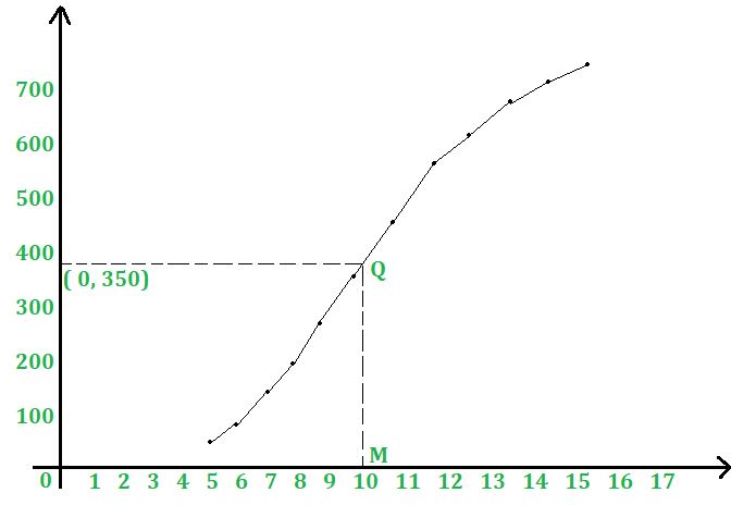
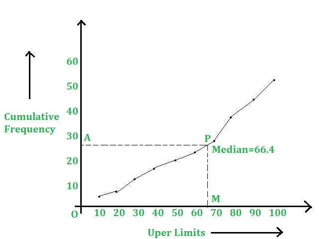
Let a grouped frequency distribution be given to us. On graph paper, we mark the upper-class limits along the x-axis and the corresponding cumulative frequencies along the y-axis. By joining these points successively by line segments, we get a polygon, called a cumulative frequency polygon. On joining these points successively by smooth curves, we get a curve, known as ogive.

The step-by-step process for the construction of an Ogive graph:

1. First, we mark the upper limits of class intervals on the horizontal x-axis and their corresponding cumulative frequencies on the y-axis.
2. Now plot all the corresponding points of the ordered pair given by (upper limit, cumulative frequency).
3. Join all the points with a free hand.
4. The curve we get is known as ogive.

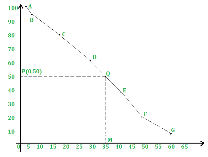
Types of Ogives

• Less Than Ogive

On graph paper, we mark the upper-class limits along the x-axis and the corresponding cumulative frequencies along the y-axis.

1. On joining these points successively by line segments, we get a polygon, called a cumulative frequency polygon.
2. On joining these points successively by smooth curves, we get a curve, known as less than ogive.

• More Than Ogive

On graph paper, we mark the lower class limits along the x-axis and the corresponding cumulative frequencies along the y-axis.

1. On joining these points successively by line segments, we get a polygon, called the cumulative frequency polygon.
2. On joining these points successively by smooth curves, we get a curve, known as more than ogive.

Check: Relation Between Mean Median and Mode

Mean, Median, and Mode of Grouped Data – FAQs

What is Grouped Data?

Grouped data is data that has been organized into groups known as classes. It is often used in statistical analysis to simplify data and focus on key trends and patterns.

How Do You Calculate the Mean of Grouped Data?

To calculate the mean of grouped data, multiply the midpoints of each class by their respective frequencies, sum these products, and then divide by the total number of data points.

Can You Find the Median in Grouped Data?

Yes, the median can be found in grouped data. It is the value that divides the dataset into two equal parts. For grouped data, the median class is identified first, and then the median value is calculated using a formula that considers the cumulative frequency.

How is the Mode Determined for Grouped Data?

The mode for grouped data is the value or class with the highest frequency. For a more precise value within a class, a modal class is identified, and the mode is calculated using a formula that accounts for the frequencies of the modal class and its adjacent classes.

Is It Possible to Calculate All Three Measures for All Types of Data?

Yes and no. Continuous data can have a mean, median, and mode calculated. Ordinal data can have a median and mode, while nominal data typically only has a mode.

Why Are These Measures Important?

Mean, median, and mode are measures of central tendency that provide insights into the distribution, concentration, and spread of data, helping in making informed decisions and comparisons.

How Do You Handle Outliers in These Calculations?

Outliers can skew the mean significantly. While the mean is sensitive to outliers, the median and mode are more robust measures that are less affected by extreme values.

Can These Measures Be Used for Comparative Analysis?

Yes, mean, median, and mode are often used to compare different datasets, such as comparing the average performance of students across different schools.

What Are the Limitations of Using Mean, Median, and Mode?

Each measure has its limitations. The mean is affected by outliers, the median may not reflect the distribution’s shape, and the mode can be ambiguous in datasets with multiple peaks.

How Do You Interpret These Measures in Real-World Data?

Interpreting these measures depends on the context. For example, the mean income of a region may give an idea of economic status, while the median can indicate the income level that divides the population into two equal groups, and the mode can show the most common income level.