MATLAB – Ideal Highpass Filter in Image Processing

In the field of Image Processing, Ideal Highpass Filter (IHPF) is used for image sharpening in the frequency domain. Image Sharpening is a technique to enhance the fine details and highlight the edges in a digital image. It removes low-frequency components from an image and preserves high-frequency components.

This ideal highpass filter is the reverse operation of the ideal lowpass filter. It can be determined using the following relation-
where, is the transfer function of the highpass filter and is the transfer function of the corresponding lowpass filter.

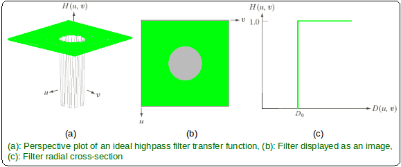
The transfer function of the IHPF can be specified by the function-

Where,

• is a positive constant. IHPF passes all the frequencies outside of a circle of radius from the origin without attenuation and cuts off all the frequencies within the circle.
• This is the transition point between H(u, v) = 1 and H(u, v) = 0, so this is termed as cutoff frequency.
• is the Euclidean Distance from any point (u, v) to the origin of the frequency plane, i.e,

Approach:

Step 1: Input – Read an image
Step 2: Saving the size of the input image in pixels
Step 3: Get the Fourier Transform of the input_image
Step 4: Assign the Cut-off Frequency
Step 5: Designing filter: Ideal High Pass Filter
Step 6: Convolution between the Fourier Transformed input image and the filtering mask
Step 7: Take Inverse Fourier Transform of the convoluted image
Step 8: Display the resultant image as output

Implementation in MATLAB:

% MATLAB Code | Ideal High Pass Filter

% Reading input image : input_image
input_image = imread('[name of input image file].[file format]');

% Saving the size of the input_image in pixels-
% M : no of rows (height of the image)
% N : no of columns (width of the image)
[M, N] = size(input_image);

% Getting Fourier Transform of the input_image
% using MATLAB library function fft2 (2D fast fourier transform)
FT_img = fft2(double(input_image));

% Assign Cut-off Frequency
D0 = 10; % one can change this value accordingly

% Designing filter
u = 0:(M-1);
idx = find(u>M/2);
u(idx) = u(idx)-M;
v = 0:(N-1);
idy = find(v>N/2);
v(idy) = v(idy)-N;

% MATLAB library function meshgrid(v, u) returns 2D grid
%  which contains the coordinates of vectors v and u.
% Matrix V with each row is a copy of v, and matrix U
% with each column is a copy of u
[V, U] = meshgrid(v, u);

% Calculating Euclidean Distance
D = sqrt(U.^2+V.^2);

% Comparing with the cut-off frequency and
% determining the filtering mask
H = double(D > D0);

% Convolution between the Fourier Transformed image and the mask
G = H.*FT_img;

% Getting the resultant image by Inverse Fourier Transform
% of the convoluted image using MATLAB library function
% ifft2 (2D inverse fast fourier transform)
output_image = real(ifft2(double(G)));

% Displaying Input Image and Output Image
subplot(2, 1, 1), imshow(input_image),
subplot(2, 1, 2), imshow(output_image, [ ]);

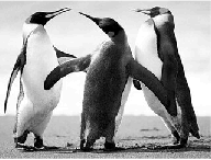
Input Image –

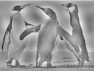
Output: