MATCH Function in Excel With Examples

Excel contains many useful functions and such a function is the ‘MATCH()’ function. It is basically used to get the relative position of a specific item from a range of cells(i.e. from a row or a column or from a table). This function also supports exact and approximate match like VLOOKUP() function. Generally, MATCH() function is used with the INDEX() function.

With the help of the MATCH() function, the user can get a relative position of a specific element from a table or range of cells. Relative position means the position of the element in the row or column where the MATCH() function is searching for the element. Precisely, this function helps us to get the position of an element in an array.

Syntax:

=MATCH(lookup_value, lookup_array, [match_type])

Here, the [match_type] value denotes if the user wants an exact match or approximate match.

Arguments:

• lookup_value (Required): It is the value(text or number or logical value or a cell reference that contains number, text or logical value) that the user wants to search. This argument must be provided by the user.
• lookup_array (Required): This argument contains the range of cells or a reference to an array where the MATCH() function will try to find out the lookup_value. Again this argument must be provided by the user.
• [match_type] (Optional): This is an optional argument. This value maybe 1, 0 or -1. If the value is 0 the user wants an exact match.  If the value is 1 MATCH() function will return the largest value that is less than or equal to lookup_value and if it is -1 the function will return the smallest value that is greater than or equal to lookup_value.

Note: If [match_type] argument is 1 or -1 then the lookup_array must be in a sorted order(ascending for 1 and descending for -1) and if the argument is not provided by the user the value becomes 1 by default.

Return Value: This function returns a value that represents the relative position of the lookup value in a range of cells.

Examples:

The example of the MATCH() function is given below. The names used in the list are only for example purposes and these are not related to any real persons.

Student Names	Age	Phone Numbers	Roll No.
Amod Yadav	21	9123456789	1010
Sukanya Tripathi	20	2345685523	1011
Vijay Chaurasia	19	1256485421	1012
Abhisekh Upmanyu	18	6665551110	1013
Dinesh Shukla	17	6026452364	1014
Vineeta Tiwari	16	2154832564	1015
Vineeta Tiwari	15	5214563254	1016
Chand Podder	14	3215648866	1017

The above list is used for example.

Formula	Result	Remarks
MATCH(A9, A1:A9, 0)	9	MATCH function searches for an exact match and returns the relative position of the element.
MATCH(1018, D1:D9)	9	Here [match_type] argument is omitted so the value is 1 and the function  searches for an approximate match and returns the position  of the next greater element in the list.
MATCH(“CHAND PODDER”, A1:A9, 0)	9	This output proves that the MATCH function is not case-sensitive.
MATCH(“Vineeta Tiwari”, A1:A9, 0)	7	MATCH function always returns the position of the first match.
MATCH(13, B1:B9, -1)	9	Here [match_type] argument is -1 and the function searches for an approximate match  and returns the position of the next smallest element in the list.

Below is the output screenshot of the Excel sheet.

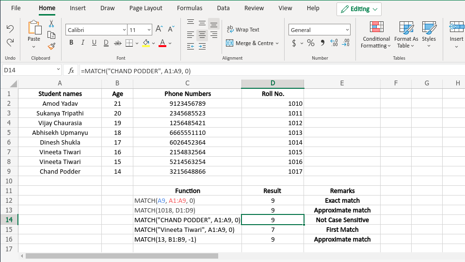
Output Screenshot