Mahotas – Zernike Features
Last Updated :
31 May, 2021
In this article we will see how we can get the zernike feature of the given image in mahotas. Zernike polynomials are an orthogonal basis set (a set of functions for which the integral of the product of any pair of functions is zero)
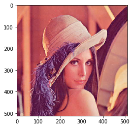
For this tutorial we will use ‘lena’ image, below is the command to load the lena image
mahotas.demos.load('lena')
Below is the lena image
In order to do this we will use mahotas.features.zernike method
Syntax : mahotas.features.zernike(img, degree, radius)
Argument : It takes image object and two integer as argument
Return : It returns 1-D array
Note : Input image should be filtered or should be loaded as grey
In order to filter the image we will take the image object which is numpy.ndarray and filter it with the help of indexing, below is the command to do this
image = image[:, :, 0]
Below is the implementation
Python3
import mahotas
import mahotas.demos
from pylab import gray, imshow, show
import numpy as np
import matplotlib.pyplot as plt
img = mahotas.demos.load('lena')
img = img.max(2)
print("Image")
imshow(img)
show()
degree = 10
radius = 10
value = mahotas.features.zernike(img, degree, radius)
print(value)
|
Output :
Image
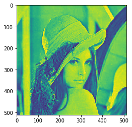
[0.31830989 0.01261485 0.00614926 0.00769591 0.0097145  0.01757332
 0.00617458 0.01008905 0.01415304 0.01099679 0.02894761 0.01838737
 0.0074247  0.01333135 0.01958184 0.00431827 0.00540781 0.01675913
 0.03511082 0.00699177 0.00357231 0.01593838 0.01621848 0.0240565
 0.0154929  0.01631347 0.03239474 0.02506811 0.00796528 0.01291179
 0.01198231 0.01916542 0.0165929  0.01032658 0.02028499 0.02506003]
Another example
Python3
import mahotas
import numpy as np
from pylab import gray, imshow, show
import os
import matplotlib.pyplot as plt
img = mahotas.imread('dog_image.png')
img = img[:, :, 0]
print("Image")
imshow(img)
show()
degree = 10
radius = 10
value = mahotas.features.zernike(img, degree, radius)
print(value)
|
Output :
Image
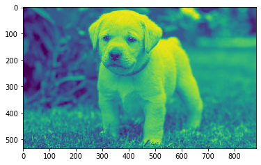
[0.31830989 0.00985427 0.00714652 0.00171408 0.00442245 0.01796711
 0.00716781 0.00179965 0.0039829  0.0031081  0.02447476 0.0011686
 0.009291   0.00174885 0.00357579 0.00692029 0.0043969  0.03528869
 0.00264739 0.01381883 0.00750501 0.0036528  0.00867514 0.01298398
 0.0129556  0.00602334 0.04108562 0.00377269 0.01859098 0.01109795
 0.00178511 0.0082474  0.01928068 0.01873102 0.00882483 0.04558572]
Like Article
Suggest improvement
Share your thoughts in the comments
Please Login to comment...