Lung Cancer Detection Using Transfer Learning

Computer Vision is one of the applications of deep neural networks that enables us to automate tasks that earlier required years of expertise and one such use in predicting the presence of cancerous cells.

In this article, we will learn how to build a classifier using the Transfer Learning technique which can classify normal lung tissues from cancerous. This project has been developed using collab and the dataset has been taken from Kaggle whose link has been provided as well.

Transfer Learning

In a convolutional neural network, the main task of the convolutional layers is to enhance the important features of an image. If a particular filter is used to identify the straight lines in an image then it will work for other images as well this is particularly what we do in transfer learning. There are models which are developed by researchers by regress hyperparameter tuning and training for weeks on millions of images belonging to 1000 different classes like imagenet dataset. A model that works well for one computer vision task proves to be good for others as well. Because of this reason, we leverage those trained convolutional layers parameters and tuned hyperparameter for our task to obtain higher accuracy.

Importing Libraries

Python libraries make it very easy for us to handle the data and perform typical and complex tasks with a single line of code.

• Pandas – This library helps to load the data frame in a 2D array format and has multiple functions to perform analysis tasks in one go.
• Numpy – Numpy arrays are very fast and can perform large computations in a very short time.
• Matplotlib – This library is used to draw visualizations.
• Sklearn – This module contains multiple libraries having pre-implemented functions to perform tasks from data preprocessing to model development and evaluation.
• OpenCV – This is an open-source library mainly focused on image processing and handling.
• Tensorflow – This is an open-source library that is used for Machine Learning and Artificial intelligence and provides a range of functions to achieve complex functionalities with single lines of code.

Python3

import numpy as np
import pandas as pd
import matplotlib.pyplot as plt
from PIL import Image
from glob import glob

from sklearn.model_selection import train_test_split
from sklearn import metrics

import cv2
import gc
import os

import tensorflow as tf
from tensorflow import keras
from keras import layers

import warnings
warnings.filterwarnings('ignore')

Importing Dataset

The dataset which we will use here has been taken from-https://www.kaggle.com/datasets/andrewmvd/lung-and-colon-cancer-histopathological-images. . This dataset includes 5000 images for three classes of lung conditions:

• Normal Class
• Lung Adenocarcinomas
• Lung Squamous Cell Carcinomas

These images for each class have been developed from 250 images by performing Data Augmentation on them. That is why we won’t be using Data Augmentation further on these images.

Python3

from zipfile import ZipFile
data_path = 'lung-and-colon-cancer-histopa\
thological-images.zip'

with ZipFile(data_path,'r') as zip:
  zip.extractall()
  print('The data set has been extracted.')

Output:

The data set has been extracted.

Data Visualization

In this section, we will try to understand visualize some images which have been provided to us to build the classifier for each class.

Python3

path = '/lung_colon_image_set/lung_image_sets'
classes = os.listdir(path)
classes

Output:

['lung_n', 'lung_aca', 'lung_scc']

These are the three classes that we have here.

Python3

path = '/lung_colon_image_set/lung_image_sets'

for cat in classes:
    image_dir = f'{path}/{cat}'
    images = os.listdir(image_dir)

    fig, ax = plt.subplots(1, 3, figsize = (15, 5))
    fig.suptitle(f'Images for {cat} category . . . .',
                 fontsize = 20)

    for i in range(3):
        k = np.random.randint(0, len(images))
        img = np.array(Image.open(f'{path}/{cat}/{images[k]}'))
        ax[i].imshow(img)
        ax[i].axis('off')
    plt.show()

Output:

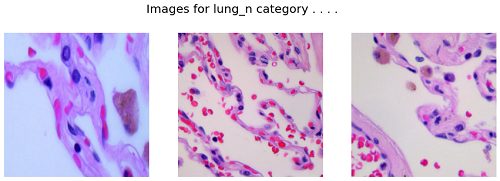
Images for lung_n category

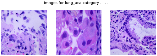
Images for lung_aca category

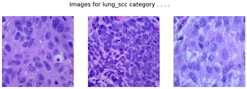
Images for lung_scc category

The above output may vary if you will run this in your notebook because the code has been implemented in such a way that it will show different images every time you rerun the code.

Data Preparation for Training

In this section, we will convert the given images into NumPy arrays of their pixels after resizing them because training a Deep Neural Network on large-size images is highly inefficient in terms of computational cost and time.

For this purpose, we will use the OpenCV library and Numpy library of python to serve the purpose. Also, after all the images are converted into the desired format we will split them into training and validation data so, that we can evaluate the performance of our model.

Python3

IMG_SIZE = 256
SPLIT = 0.2
EPOCHS = 10
BATCH_SIZE = 64

Some of the hyperparameters we can tweak from here for the whole notebook.

Python3

X = []
Y = []

for i, cat in enumerate(classes):
  images = glob(f'{path}/{cat}/*.jpeg')

  for image in images:
    img = cv2.imread(image)

    X.append(cv2.resize(img, (IMG_SIZE, IMG_SIZE)))
    Y.append(i)

X = np.asarray(X)
one_hot_encoded_Y = pd.get_dummies(Y).values

One hot encoding will help us to train a model which can predict soft probabilities of an image being from each class with the highest probability for the class to which it really belongs.

Python3

X_train, X_val, Y_train, Y_val = train_test_split(
  X, one_hot_encoded_Y, test_size = SPLIT, random_state = 2022)
print(X_train.shape, X_val.shape)

Output:

(12000, 256, 256, 3) (3000, 256, 256, 3)

In this step, we will achieve the shuffling of the data automatically because the train_test_split function split the data randomly in the given ratio.

Model Development

We will use pre-trained weight for an Inception network which is trained on imagenet dataset. This dataset contains millions of images for around 1000 classes of images.

Model Architecture

We will implement a model using the  Functional API of Keras which will contain the following parts:

• The base model is the Inception model in this case.
• The Flatten layer flattens the output of the base model’s output.
• Then we will have two fully connected layers followed by the output of the flattened layer.
• We have included some BatchNormalization layers to enable stable and fast training and a Dropout layer before the final layer to avoid any possibility of overfitting.
• The final layer is the output layer which outputs soft probabilities for the three classes. 

Python3

from tensorflow.keras.applications.inception_v3 import InceptionV3

pre_trained_model = InceptionV3(
    input_shape = (IMG_SIZE, IMG_SIZE, 3),
    weights = 'imagenet',
    include_top = False
)

Output:

87916544/87910968 [==============================] – 2s 0us/step

87924736/87910968 [==============================] – 2s 0us/step

Python3

len(pre_trained_model.layers)

Output:

311

This is how deep this model is this also justifies why this model is highly effective in extracting useful features from images which helps us to build classifiers.

The parameters of a model we import are already trained on millions of images and for weeks so, we do not need to train them again.

Python3

for layer in pre_trained_model.layers:
  layer.trainable = False

‘Mixed7’ is one of the layers in the inception network whose outputs we will use to build the classifier.

Python3

last_layer = pre_trained_model.get_layer('mixed7')
print('last layer output shape: ', last_layer.output_shape)
last_output = last_layer.output

Output:

last layer output shape:  (None, 14, 14, 768)

Python3

x = layers.Flatten()(last_output)

x = layers.Dense(256,activation='relu')(x)
x = layers.BatchNormalization()(x)

x = layers.Dense(128,activation='relu')(x)
x = layers.Dropout(0.3)(x)
x = layers.BatchNormalization()(x)

output = layers.Dense(3, activation='softmax')(x)

model = keras.Model(pre_trained_model.input, output)

While compiling a model we provide these three essential parameters:

• optimizer – This is the method that helps to optimize the cost function by using gradient descent.
• loss – The loss function by which we monitor whether the model is improving with training or not.
• metrics – This helps to evaluate the model by predicting the training and the validation data.

Python3

model.compile(
    optimizer='adam',
    loss='categorical_crossentropy',
    metrics=['accuracy']
)

Callback

Callbacks are used to check whether the model is improving with each epoch or not. If not then what are the necessary steps to be taken like ReduceLROnPlateau decreases the learning rate further? Even then if model performance is not improving then training will be stopped by EarlyStopping. We can also define some custom callbacks to stop training in between if the desired results have been obtained early.

Python3

from keras.callbacks import EarlyStopping, ReduceLROnPlateau

class myCallback(tf.keras.callbacks.Callback):
  def on_epoch_end(self, epoch, logs = {}):
    if logs.get('val_accuracy') > 0.90:
      print('\n Validation accuracy has reached upto 90%\
      so, stopping further training.')
      self.model.stop_training = True

es = EarlyStopping(patience = 3,
                   monitor = 'val_accuracy',
                   restore_best_weights = True)

lr = ReduceLROnPlateau(monitor = 'val_loss',
                       patience = 2,
                       factor = 0.5,
                       verbose = 1)

Now we will train our model:

Python3

history = model.fit(X_train, Y_train,
                    validation_data = (X_val, Y_val),
                    batch_size = BATCH_SIZE,
                    epochs = EPOCHS,
                    verbose = 1,
                    callbacks = [es, lr, myCallback()])

Output:

Model training progress

Let’s visualize the training and validation accuracy with each epoch.

Python3

history_df = pd.DataFrame(history.history)
history_df.loc[:,['loss','val_loss']].plot()
history_df.loc[:,['accuracy','val_accuracy']].plot()
plt.show()

Output:

Graph of loss and accuracy epoch by epoch for training and validation data.loss

From the above graphs, we can certainly say that the model has not overfitted the training data as the difference between the training and validation accuracy is very low.

Model Evaluation

Now as we have our model ready let’s evaluate its performance on the validation data using different metrics. For this purpose, we will first predict the class for the validation data using this model and then compare the output with the true labels.

Python3

Y_pred = model.predict(X_val)

Y_val = np.argmax(Y_val, axis=1)
Y_pred = np.argmax(Y_pred, axis=1)

Let’s draw the confusion metrics and classification report using the predicted labels and the true labels.

Python3

metrics.confusion_matrix(Y_val, Y_pred)

Output:

Confusion matrix for the validation data

Python3

print(metrics.classification_report(Y_val, Y_pred,
                                    target_names=classes))

Output:

Classification report for the validation data

Conclusion: Indeed the performance of our model using the Transfer Learning Technique has achieved higher accuracy without overfitting which is very good as the f1-score for each class is also above 0.90 which means our model’s prediction is correct 90% of the time.