Level Ordering of Factors in R Programming
Last Updated :
08 Jun, 2023
In this article, we will see the level ordering of factors in the R Programming Language.
R – Level Ordering of Factors
Factors are data objects used to categorize data and store it as levels. They can store a string as well as an integer. They represent columns as they have a limited number of unique values. Factors in R can be created using the factor() function. It takes a vector as input. c() function is used to create a vector with explicitly provided values.
Example:
R
x <- c("Pen", "Pencil", "Brush", "Pen",
"Brush", "Brush", "Pencil", "Pencil")
print(x)
print(is.factor(x))
factor_x = factor(x)
levels(factor_x)
|
Output :
[1] "Pen"    "Pencil" "Brush"  "Pen"    "Brush"  "Brush"  "Pencil" "Pencil"

[1] FALSE

[1] "Brush"  "Pen"    "Pencil"
In the above code, x is a vector with 8 elements. To convert it to a factor the function factor() is used. Here there are 8 factors and 3 levels. Levels are the unique elements in the data. It can be found using the levels() function.
Ordering Factor Levels
Ordered factors levels are an extension of factors. It arranges the levels in increasing order. We use two functions: factor() and argument ordered().
Syntax: factor(data, levels =c(“”), ordered =TRUE)
Parameter:
- data: input vector with explicitly defined values.
- levels(): Mention the list of levels in c function.
- ordered: It is set true for enabling ordering.
Example:
R
size = c("small", "large", "large", "small",
"medium", "large", "medium", "medium")
size_factor <- factor(size)
print(size_factor)
ordered.size <- factor(size, levels = c(
"small", "medium", "large"), ordered = TRUE)
print(ordered.size)
|
Output:
[1] small  large  large  small  medium large  medium medium
Levels: large medium small

[1] small  large  large  small  medium large  medium medium
Levels: small < medium < large
In the above code, the size vector is created using the c function. Then it is converted to a factor. And for the ordering factor, the () function is used along with the arguments described above. Thus the sizes are arranged in order.
The same can be done using the ordered function. An example of the same is shown below:
Example:
R
size = c("small", "large", "large", "small",
"medium", "large", "medium", "medium")
sizes <- ordered(c("small", "large", "large",
"small", "medium"))
sizes <- ordered(sizes, levels = c("small", "medium", "large"))
print(sizes)
|
Output:
[1] small  large  large  small  medium
Levels: small < medium < large
Level ordering visualization in R
we have a dataset of student grades, and we want to create a boxplot to compare the distribution of grades for different class levels (freshman, sophomore, junior, and senior). We can create a factor variable to represent the class levels and specify the level ordering so that the boxplot is ordered by class level.
Example:
R
grades <- data.frame(
grade = c(75, 82, 68, 92, 89, 78, 85, 90, 72, 81, 94, 87, 79, 86, 91),
level = factor(c(rep("freshman", 5), rep("sophomore", 4), rep("junior", 3), rep("senior", 3)))
)
grades$level <- factor(grades$level, levels = c("freshman", "sophomore", "junior", "senior"))
boxplot(grade ~ level, data = grades, main = "Student Grades by Class Level")
|
Output:
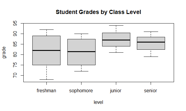
Level Ordering of Factors in R Programming
In this example, we create a sample dataset of student grades with a grade column and a level column representing the class level of each student. We then create a factor variable level from the level column and specify the level ordering as “freshman”, “sophomore”, “junior”, and “senior” using the factor() function.
Finally, we create a boxplot of grades by class level using the boxplot() function. The grade column represents the response variable, and the level column represents the explanatory variable. We also specify a title for the plot.
As you can see, the boxplot is ordered by class level according to our specified level ordering, with the freshman grades on the left and the senior grades on the right. This makes it easier to compare the distribution of grades for each class level. If we had not specified the level order, R would have used the default alphabetical ordering (“freshman”, “junior”, “senior”, “sophomore”), which would not have been as useful for visualizing the data.
Share your thoughts in the comments
Please Login to comment...