Ledoit-Wolf vs OAS Estimation in Scikit Learn

Generally, Shrinkage is used to regularize the usual covariance maximum likelihood estimation. Ledoit and Wolf proposed a formula which is known as the Ledoit-Wolf covariance estimation formula; This close formula can compute the asymptotically optimal shrinkage parameter with minimizing a Mean Square Error(MSE) criterion feature. After that, one researcher Chen et al. made improvements in the Ledoit-Wolf Shrinkage parameter. He proposed Oracle Approximating Shrinkage (OAS) coefficient whose convergence is significantly better under the assumption that the data are Gaussian.

There are some basic concepts are needed  to develop the Ledoit-Wolf estimators given below  step by step:

Importing Libraries and Setting up the Variables

Python libraries make it very easy for us to handle the data and perform typical and complex tasks with a single line of code.

• Numpy – Numpy arrays are very fast and can perform large computations in a very short time.
• Matplotlib/Seaborn – This library is used to draw visualizations.
• Sklearn – This module contains multiple libraries having pre-implemented functions to perform tasks from data preprocessing to model development and evaluation.
• Scipy – SciPy is a python library that is useful in solving many mathematical equations and algorithms at its core it uses NumPy to handle the numbers.

Python3

# importing necessary libraries
import numpy as np
from sklearn.covariance import LedoitWolf, OAS
from scipy.linalg import toeplitz, cholesky
import matplotlib.pyplot as plt

# creating seeds for high productivity
np.random.seed(0)
numOffeatures = 250

# Simulation Covariance Matrix
r = 0.25
# covariance estimation
realTimeCovariance = toeplitz(r ** np.arange(numOffeatures))
# matrix generation
colorMatrix = cholesky(realTimeCovariance)

Creating Variables to Store Results

Now we will initialize some NumPy matrices so, that we can store the results from the estimation to them. Here, the mean squared error calculation logic and shrinkage estimation logic of both Ledoit-Wolf and OAS is being specified.

Python3

# specifying the sampling range
numOfSamplesRange = np.arange(8, 40, 1)
repeat = 150
# MSE logic specification
ledoitWolf_mse = np.zeros((numOfSamplesRange.size, repeat))
oas_mse = np.zeros((numOfSamplesRange.size, repeat))
# shrinkage estimation
ledoitWolf_shrinkage = np.zeros((numOfSamplesRange.size, repeat))
oas_shrinkage = np.zeros((numOfSamplesRange.size, repeat))

Parameters

• Store_precision: bool, default=True 
• Assume_centered: bool, default=False
• Block_size: int, default=1000 

Attributes

• Covariance_: array of shape (n_features, n_features)
• Precision_: array of shape (n_features, n_features)
• shrinkage_: float
• n_features_in_: int

Now, we will calculate the MSE and shrinkage by using nested for loop to fit the values for both models step by step:

Python3

# defining nested loop for each step iteration
for i, numOfSamples in enumerate(numOfSamplesRange):
    for j in range(repeat):
        X = np.dot(np.random.normal(size=(numOfSamples, numOffeatures)),
                   colorMatrix.T)
# calculation of MSE and shrinkage for Ledoit-Wolf model
        ledoitWolf = LedoitWolf(store_precision=False,
                                assume_centered=True)
        ledoitWolf.fit(X) #fitting the values in model
        ledoitWolf_mse[i, j] = ledoitWolf.error_norm(realTimeCovariance,
                                                     scaling=False) # error normalization
        ledoitWolf_shrinkage[i, j] = ledoitWolf.shrinkage_
# calculation of MSE and shrinkage for OAS  model
        oas = OAS(store_precision=False, assume_centered=True)
        oas.fit(X)    #fitting the values in model
        oas_mse[i, j] = oas.error_norm(realTimeCovariance,
                                       scaling=False)  # error normalization
        oas_shrinkage[i, j] = oas.shrinkage_

Visualizing MSE and Shrinkage

Now let’s create a graph for both of the estimations first for error and then for shrinkage. Here, graphs for the comparison between Ledoit-Wolf and OAS have been plotted in the factor of MSE and shrinkage accordingly.

Python3

# plotting Mean Square Error(MSE)
# error plotting for Ledoit-Wolf
plt.subplot(2, 1, 1)
plt.errorbar(
    numOfSamplesRange,
    ledoitWolf_mse.mean(1), yerr=ledoitWolf_mse.std(1),
    label="Ledoit-Wolf", color="yellow", lw=2,
)

# error plotting for OAS coefficient
plt.errorbar(
    numOfSamplesRange,
    oas_mse.mean(1), yerr=oas_mse.std(1),
    label="OAS", color="green", lw=2,
)

plt.ylabel("Squared error")
plt.legend(loc="upper right")
plt.title("Comparison of covariance estimators(Ledoit-Wolf vs OAS)")
plt.xlim(2, 32)
plt.show()

Output:

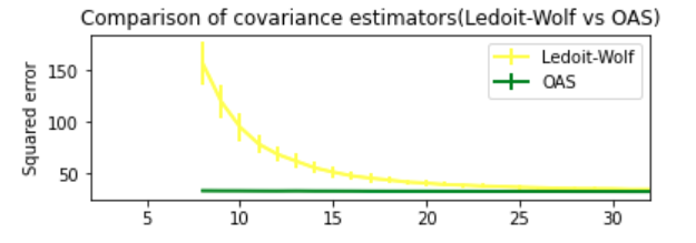
Ledoit-Wolf vs OAS (comparison factor is MSE)

Python3

# plot Shrinkage coefficient
# Shrinkage plotting for Ledoit-Wolf
plt.subplot(2, 1, 2)
plt.errorbar(
    numOfSamplesRange,
    ledoitWolf_shrinkage.mean(1), yerr=ledoitWolf_shrinkage.std(1),
    label="Ledoit-Wolf", color="yellow", lw=2,
)

# Shrinkage plotting for OAS coefficient
plt.errorbar(
    numOfSamplesRange,
    oas_shrinkage.mean(1), yerr=oas_shrinkage.std(1),
    label="OAS", color="green", lw=2,
)

plt.xlabel("number of samples")
plt.ylabel("Shrinkage counting")
plt.legend(loc="lower right")
plt.ylim(plt.ylim()[0], 1.0 + (plt.ylim()[1] - plt.ylim()[0]) / 10.0)
plt.xlim(2, 32)
plt.show()

Output:

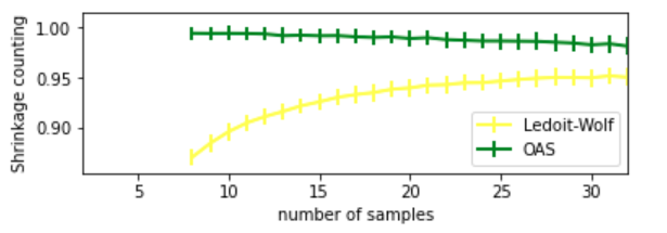
Ledoit-Wolf vs OAS (comparison factor is shrinkage)