R is a Programming Language that is mostly used for machine learning, data analysis, and statistical computing. It is an interpreted language and is platform independent that means it can be used on platforms like Windows, Linux, and macOS.

In this R Language tutorial, we will Learn R Programming Language from scratch to advance and this tutorial is suitable for both beginners and experienced developers).
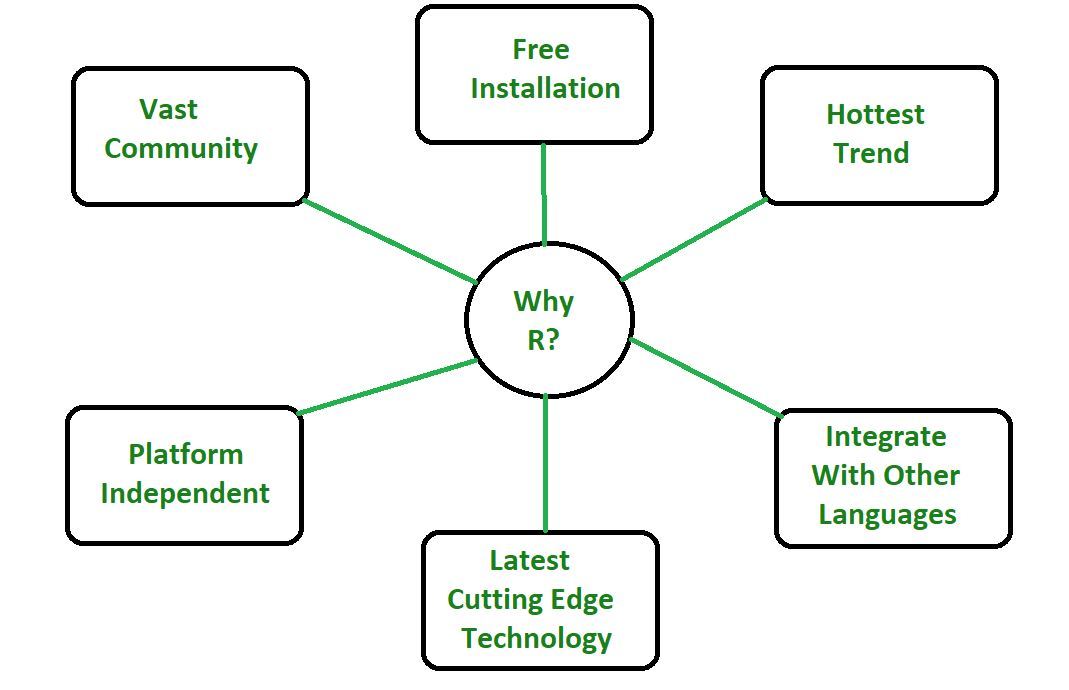
Why Learn R Programming Language?
- R programming is used as a leading tool for machine learning, statistics, and data analysis.
- R is an open-source language that means it is free of cost and anyone from any organization can install it without purchasing a license.
- It is available across widely used platforms like windows, Linux, and macOS.
- R programming language is not only a statistic package but also allows us to integrate with other languages (C, C++). Thus, you can easily interact with many data sources and statistical packages.
- Its user base is growing day by day and has vast community support.
- R Programming Language is currently one of the most requested programming languages in the Data Science job market that makes it the hottest trend nowadays.
Key Features and Applications
Some key features of R that make the R one of the most demanding job in data science market are:
- Basic Statistics: The most common basic statistics terms are the mean, mode, and median. These are all known as “Measures of Central Tendency.” So using the R language we can measure central tendency very easily.
- Static graphics: R is rich with facilities for creating and developing various kinds of static graphics including graphic maps, mosaic plots, biplots, and the list goes on.
- Probability distributions: Using R we can easily handle various types of probability distribution such as Binomial Distribution, Normal Distribution, Chi-squared Distribution, and many more.
- R Packages: One of the major features of R is it has a wide availability of libraries. R has CRAN(Comprehensive R Archive Network), which is a repository holding more than 10,0000 packages.
- Distributed Computing: Distributed computing is a model in which components of a software system are shared among multiple computers to improve efficiency and performance. Two new packages ddR and multidplyr used for distributed programming in R were released in November 2015.
Applications of R

Download and Installation
There are many IDE’s available for using R in this article we will dealing with the installation of RStudio in R.
Refer to the below articles to get detailed information about RStudio and its installation.
Hello World in R
R Program can be run in several ways. You can choose any of the following options to continue with this tutorial.
- Using IDEs like RStudio, Eclipse, Jupyter, Notebook, etc.
- Using R Command Prompt
- Using RScripts
Now type the below code to print hello world on your console.
Output:
[1] "HelloWorld"
Note: For more information, refer Hello World in R Programming
Fundamentals of R
Variables:
R is a dynamically typed language, i.e. the variables are not declared with a data type rather they take the data type of the R-object assigned to them. In R, the assignment can be denoted in three ways.
- Using equal operator- data is copied from right to left.
variable_name = value
- Using leftward operator- data is copied from right to left.
variable_name <- value
- Using rightward operator- data is copied from left to right.
value -> variable_name
Example:
R
var1 = "gfg"
print(var1)
var2 <- "gfg"
print(var2)
"gfg" -> var3
print(var3)
|
Output:
[1] "gfg"
[1] "gfg"
[1] "gfg"
Note: For more information, refer R – Variables.
Comments:
Comments are the english sentences that are used to add useful information to the source code to make it more understandable by the reader. It explains the logic part used in the code and will have no impact in the code during its execution. Any statement starting with “#” is a comment in R.
Example:
R
a <- 1
b <- 2
print(a + b)
|
Output:
[1] 3
Note: For more information, refer Comments in R
Operators
Operators are the symbols directing the various kinds of operations that can be performed between the operands. Operators simulate the various mathematical, logical and decision operations performed on a set of Complex Numbers, Integers, and Numericals as input operands. These are classified based on their functionality –
- Arithmetic Operators: Arithmetic operations simulate various math operations, like addition, subtraction, multiplication, division and modulo.
Example:
R
a <- 12
b <- 5
cat ("Addition :", a + b, "\n")
cat ("Subtraction :", a - b, "\n")
cat ("Multiplication :", a * b, "\n")
cat ("Division :", a / b, "\n")
cat ("Modulo :", a %% b, "\n")
cat ("Power operator :", a ^ b)
|
Output:
Addition : 17
Subtraction : 7
Multiplication : 60
Division : 2.4
Modulo : 2
Power operator : 248832
- Logical Operators: Logical operations simulate element-wise decision operations, based on the specified operator between the operands, which are then evaluated to either a True or False boolean value.
Example:
R
vec1 <- c(FALSE, TRUE)
vec2 <- c(TRUE,FALSE)
cat ("Element wise AND :", vec1 & vec2, "\n")
cat ("Element wise OR :", vec1 | vec2, "\n")
cat ("Logical AND :", vec1 && vec2, "\n")
cat ("Logical OR :", vec1 || vec2, "\n")
cat ("Negation :", !vec1)
|
Output:
Element wise AND : FALSE FALSE
Element wise OR : TRUE TRUE
Logical AND : FALSE
Logical OR : TRUE
Negation : TRUE FALSE
- Relational Operators: The relational operators carry out comparison operations between the corresponding elements of the operands.
Example:
R
a <- 10
b <- 14
cat ("a less than b :", a < b, "\n")
cat ("a less than equal to b :", a <= b, "\n")
cat ("a greater than b :", a > b, "\n")
cat ("a greater than equal to b :", a >= b, "\n")
cat ("a not equal to b :", a != b, "\n")
|
Output:
a less than b : TRUE
a less than equal to b : TRUE
a greater than b : FALSE
a greater than equal to b : FALSE
a not equal to b : TRUE
- Assignment Operators: Assignment operators are used to assign values to various data objects in R.
Example:
R
v1 <- "GeeksForGeeks"
v2 <<- "GeeksForGeeks"
v3 = "GeeksForGeeks"
"GeeksForGeeks" ->> v4
"GeeksForGeeks" -> v5
cat("Value 1 :", v1, "\n")
cat("Value 2 :", v2, "\n")
cat("Value 3 :", v3, "\n")
cat("Value 4 :", v4, "\n")
cat("Value 5 :", v5)
|
Output:
Value 1 : GeeksForGeeks
Value 2 : GeeksForGeeks
Value 3 : GeeksForGeeks
Value 4 : GeeksForGeeks
Value 5 : GeeksForGeeks
Note: For more information, refer R – Operators
Keywords:
Keywords are specific reserved words in R, each of which has a specific feature associated with it. Here is the list of keywords in R:
| if |
function |
FALSE |
NA_integer |
| else |
in |
NULL |
NA_real |
| while |
next |
Inf |
NA_complex_ |
| repeat |
break |
NaN |
NA_character_ |
| for |
TRUE |
NA |
… |
Note: For more information, refer R – Keywords
Data Types
Each variable in R has an associated data type. Each data type requires different amounts of memory and has some specific operations which can be performed over it. R supports 5 type of data types. These are –
| Data Types |
Example |
Description |
| Numeric |
1, 2, 12, 36 |
Decimal values are called numerics in R. It is the default data type for numbers in R. |
| Integer |
1L, 2L, 34L |
R supports integer data types which are the set of all integers. Capital ‘L’ notation as a suffix is used to denote that a particular value is of the integer data type. |
| Logical |
TRUE, FALSE |
Take either a value of true or false |
| Complex |
2+3i, 5+7i |
Set of all the complex numbers. The complex data type is to store numbers with an imaginary component. |
| Character |
‘a’, ’12’, “GFG”, ”’hello”’ |
R supports character data types where you have all the alphabets and special characters. |
Example:
R
print("Numberic type")
x = 12.25
print(class(x))
print(typeof(x))
print("----------------------------")
print("Integer Type")
y = 15L
print(class(y))
print(typeof(y))
print("----------------------------")
print("Logical Type")
x = 1
y = 2
z = x > y
print(z)
print(class(z))
print(typeof(z))
print("----------------------------")
print("Complex Type")
x = 12 + 13i
print(class(x))
print(typeof(x))
print("----------------------------")
print("Character Type")
char = "GFG"
print(class(char))
print(typeof(char))
|
Output:
[1] "Numberic type"
[1] "numeric"
[1] "double"
[1] "----------------------------"
[1] "Integer Type"
[1] "integer"
[1] "integer"
[1] "----------------------------"
[1] "Logical Type"
[1] TRUE
[1] "logical"
[1] "logical"
[1] "----------------------------"
[1] "Complex Type"
[1] "complex"
[1] "complex"
[1] "----------------------------"
[1] "Character Type"
[1] "character"
[1] "character"
Note: for more information, refer R – Data Types
Basics of Input/Output
Taking Input from the User:
R Language provides us with two inbuilt functions to read the input from the keyboard.
- readline() method: It takes input in string format. If one inputs an integer then it is inputted as a string.
Example:
- scan() method: This method reads data in the form of a vector or list. This method is a very handy method while inputs are needed to taken quickly for any mathematical calculation or for any dataset.
Example:
Note: For more information, refer Taking Input from User in R Programming
Printing Output to Console:
R Provides various functions to write output to the screen, let’s see them –
- print(): It is the most common method to print the output.
Example:
R
print("Hello")
x <- "Welcome to GeeksforGeeks"
print(x)
|
Output:
[1] "Hello"
[1] "Welcome to GeeksforGeeks"
- cat(): cat() converts its arguments to character strings. This is useful for printing output in user defined functions.
Example:
R
x = "Hello"
cat(x, "\nwelcome")
cat("\nto GeeksForGeeks")
|
Output:
Hello
welcome
to GeeksForGeeks
Note: For more information, refer Printing Output of an R Program
Decision Making
Decision making decides the flow of the execution of the program based on certain conditions. In decision making programmer needs to provide some condition which is evaluated by the program, along with it there also provided some statements which are executed if the condition is true and optionally other statements if the condition is evaluated to be false.
Decision-making statements in R Language:
Example 1: Demonstrating if and if-else
R
a <- 99
b <- 12
if(a > b)
{
print("A is Larger")
}
if(b > a)
{
print("B is Larger")
} else
{
print("A is Larger")
}
|
Output:
[1] "A is Larger"
[1] "A is Larger"
Example 2: Demonstrating if-else-if and nested if
R
a <- 10
if (a == 11)
{
print ("a is 11")
} else if (a==10)
{
print ("a is 10")
} else
print ("a is not present")
if (a %% 2 == 0)
{
if (a %% 5 == 0)
print("Number is divisible by both 2 and 5")
}
|
Output:
[1] "a is 10"
[1] "Number is divisible by both 2 and 5"
Example 3: Demonstrating switch
R
x <- switch(
2,
"Welcome",
"to",
"GFG"
)
print(x)
y <- switch(
"3",
"0"="Welcome",
"1"="to",
"3"="GFG"
)
print(y)
z <- switch(
"GfG",
"GfG0"="Welcome",
"GfG1"="to",
"GfG3"="GFG"
)
print(z)
|
Output:
[1] "to"
[1] "GFG"
NULL
Note: For more information, refer Decision Making in R Programming
Control Flow
Loops are used wherever we have to execute a block of statements repeatedly. For example, printing “hello world” 10 times. The different types of loops in R are –
Example:
R
for (i in c(-8, 9, 11, 45))
{
print(i)
}
|
Output:
[1] -8
[1] 9
[1] 11
[1] 45
Example:
R
val = 1
while (val <= 5 )
{
print(val)
val = val + 1
}
|
Output:
[1] 1
[1] 2
[1] 3
[1] 4
[1] 5
Example:
R
val = 1
repeat
{
print(val)
val = val + 1
if(val > 5)
{
break
}
}
|
Output:
[1] 1
[1] 2
[1] 3
[1] 4
[1] 5
Note: For more information, refer Loops in R
Loop Control Statements
Loop control statements change execution from its normal sequence. Following are the loop control statements provided by R Language:
- Break Statement: The break keyword is a jump statement that is used to terminate the loop at a particular iteration.
- Next Statement: The next statement is used to skip the current iteration in the loop and move to the next iteration without exiting from the loop itself.
R
no <- 15:20
for (val in no)
{
if (val == 17)
{
break
}
print(paste("Values are: ", val))
}
print("------------------------------------")
for (val in no)
{
if (val == 17)
{
next
}
print(paste("Values are: ", val))
}
|
Output:
[1] "Values are:  15"
[1] "Values are:  16"
[1] "------------------------------------"
[1] "Values are:  15"
[1] "Values are:  16"
[1] "Values are:  18"
[1] "Values are:  19"
[1] "Values are:  20"
Note: For more information, refer Break and Next statements in R
Functions
Functions are the block of code that given the user the ability to reuse the same code which saves the excessive use of memory and provides better readability to the code. So basically, a function is a collection of statements that perform some specific task and return the result to the caller. Functions are created in R by using the command function() keyword
Example:
R
ask_user = function(x){
print("GeeksforGeeks")
}
my_func = function(x){
a <- 1:5
b <- 0
for (i in a){
b = b +1
}
return(b)
}
ask_user()
res = my_func()
print(res)
|
Output:
[1] "GeeksforGeeks"
[1] 5
Function with Arguments:
Arguments to a function can be specified at the time of function definition, after the function name, inside the parenthesis.
Example:
R
evenOdd = function(x){
if(x %% 2 == 0)
return("even")
else
return("odd")
}
divisible <- function(a, b){
if(a %% b == 0)
{
cat(a, "is divisible by", b, "\n")
} else
{
cat(a, "is not divisible by", b, "\n")
}
}
print(evenOdd(4))
print(evenOdd(3))
divisible(7, 3)
divisible(36, 6)
divisible(9, 2)
|
Output:
[1] "even"
[1] "odd"
7 is not divisible by 3
36 is divisible by 6
9 is not divisible by 2
- Default Arguments: Default value in a function is a value that is not required to specify each time the function is called.
Example:
R
isdivisible <- function(a, b = 9){
if(a %% b == 0)
{
cat(a, "is divisible by", b, "\n")
} else
{
cat(a, "is not divisible by", b, "\n")
}
}
isdivisible(20, 2)
isdivisible(12)
|
Output:
20 is divisible by 2
12 is not divisible by 9
- Variable length arguments: Dots argument (…) is also known as ellipsis which allows the function to take an undefined number of arguments.
Example:
R
fun <- function(n, ...){
l <- c(n, ...)
paste(l, collapse = " ")
}
fun(5, 1L, 6i, TRUE, "GFG", 1:2)
|
Output:
5 1 0+6i TRUE GFG 1 2
Refer to the below articles to get detailed information about functions in R
Data Structures
A data structure is a particular way of organizing data in a computer so that it can be used effectively.
Vectors:
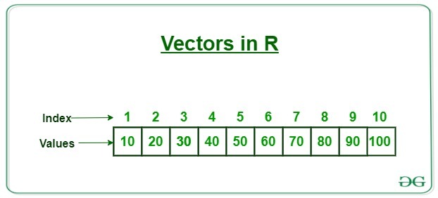
Vectors in R are the same as the arrays in C language which are used to hold multiple data values of the same type. One major key point is that in R the indexing of the vector will start from ‘1’ and not from ‘0’.
Example:
R
N = c(1, 3, 5, 7, 8)
C = c('Geeks', 'For', 'Geeks')
L = c(TRUE, FALSE, FALSE, TRUE)
print(N)
print(C)
print(L)
|
Output:
[1] 1 3 5 7 8
[1] "Geeks" "For"   "Geeks"
[1]  TRUE FALSE FALSE  TRUE
Accessing Vector Elements:
There are many ways through which we can access the elements of the vector. The most common is using the ‘[]’, symbol.
Example:
R
X <- c(2, 9, 8, 0, 5)
print('using Subscript operator')
print(X[2])
Y <- c(6, 2, 7, 4, 0)
print('using c function')
print(Y[c(4, 1)])
Z <- c(1, 6, 9, 4, 6)
print('Logical indexing')
print(Z[Z>3])
|
Output:
[1] "using Subscript operator"
[1] 9
[1] "using c function"
[1] 4 6
[1] "Logical indexing"
[1] 6 9 4 6
Refer to the below articles to get detailed information about vectors in R.
Lists:
A list is a generic object consisting of an ordered collection of objects. Lists are heterogeneous data structures.
Example:
R
empId = c(1, 2, 3, 4)
empName = c("Nisha", "Nikhil", "Akshu", "Sambha")
numberOfEmp = 4
Organization = "GFG"
empList = list(empId, empName, numberOfEmp, Organization)
print(empList)
|
Output:
[[1]]
[1] 1 2 3 4

[[2]]
[1] "Nisha"  "Nikhil" "Akshu"  "Sambha"

[[3]]
[1] 4

[[4]]
[1] "GFG"
Accessing List Elements:
- Access components by names: All the components of a list can be named and we can use those names to access the components of the list using the dollar command.
- Access components by indices: We can also access the components of the list using indices. To access the top-level components of a list we have to use a double slicing operator “[[ ]]” which is two square brackets and if we want to access the lower or inner level components of a list we have to use another square bracket “[ ]” along with the double slicing operator “[[ ]]“.
Example:
R
empId = c(1, 2, 3, 4)
empName = c("Nisha", "Nikhil", "Akshu", "Sambha")
numberOfEmp = 4
empList = list(
"ID" = empId,
"Names" = empName,
"Total Staff" = numberOfEmp
)
print("Initial List")
print(empList)
cat("\nAccessing name components using $ command\n")
print(empList$Names)
cat("\nAccessing name components using indices\n")
print(empList[[2]])
print(empList[[1]][2])
print(empList[[2]][4])
|
Output:
[1] "Initial List"
$ID
[1] 1 2 3 4

$Names
[1] "Nisha"  "Nikhil" "Akshu"  "Sambha"

$`Total Staff`
[1] 4


Accessing name components using $ command
[1] "Nisha"  "Nikhil" "Akshu"  "Sambha"

Accessing name components using indices
[1] "Nisha"  "Nikhil" "Akshu"  "Sambha"
[1] 2
[1] "Sambha"
Adding and Modifying list elements:
- A list can also be modified by accessing the components and replacing them with the ones which you want.
- List elements can be added simply by assigning new values using new tags.
Example:
R
empId = c(1, 2, 3, 4)
empName = c("Nisha", "Nikhil", "Akshu", "Sambha")
numberOfEmp = 4
empList = list(
"ID" = empId,
"Names" = empName,
"Total Staff" = numberOfEmp
)
print("Initial List")
print(empList)
empList[["organization"]] <- "GFG"
cat("\nAfter adding new element\n")
print(empList)
empList$"Total Staff" = 5
empList[[1]][5] = 7
cat("\nAfter modification\n")
print(empList)
|
Output:
[1] "Initial List"
$ID
[1] 1 2 3 4

$Names
[1] "Nisha"  "Nikhil" "Akshu"  "Sambha"

$`Total Staff`
[1] 4


After adding new element
$ID
[1] 1 2 3 4

$Names
[1] "Nisha"  "Nikhil" "Akshu"  "Sambha"

$`Total Staff`
[1] 4

$organization
[1] "GFG"


After modification
$ID
[1] 1 2 3 4 7

$Names
[1] "Nisha"  "Nikhil" "Akshu"  "Sambha"

$`Total Staff`
[1] 5

$organization
[1] "GFG"
Refer to the below articles to get detailed information about lists in R
Matrices:
A matrix is a rectangular arrangement of numbers in rows and columns. Matrices are two-dimensional, homogeneous data structures.
Example:
R
A = matrix(
c(1, 4, 5, 6, 3, 8),
nrow = 2, ncol = 3,
byrow = TRUE
)
print(A)
|
Output:
     [,1] [,2] [,3]
[1,]    1    4    5
[2,]    6    3    8
Accessing Matrix Elements:
Matrix elements can be accessed using the matrix name followed by a square bracket with a comma in between the array. Value before the comma is used to access rows and value that is after the comma is used to access columns.
Example:
R
A = matrix(
c(1, 4, 5, 6, 3, 8),
nrow = 2, ncol = 3,
byrow = TRUE
)
cat("The 2x3 matrix:\n")
print(A)
print(A[1, 1])
print(A[2, 2])
cat("Accessing first and second row\n")
print(A[1:2, ])
cat("\nAccessing first and second column\n")
print(A[, 1:2])
|
Output:
The 2x3 matrix:
     [,1] [,2] [,3]
[1,]    1    4    5
[2,]    6    3    8
[1] 1
[1] 3
Accessing first and second row
     [,1] [,2] [,3]
[1,]    1    4    5
[2,]    6    3    8

Accessing first and second column
     [,1] [,2]
[1,]    1    4
[2,]    6    3
Modifying Matrix Elements:
You can modify the elements of the matrices by a direct assignment.
Example:
R
A = matrix(
c(1, 4, 5, 6, 3, 8),
nrow = 2,
ncol = 3,
byrow = TRUE
)
cat("The 2x3 matrix:\n")
print(A)
A[2, 1] = 30
cat("After edited the matrix\n")
print(A)
|
Output:
The 2x3 matrix:
     [,1] [,2] [,3]
[1,]    1    4    5
[2,]    6    3    8
After edited the matrix
     [,1] [,2] [,3]
[1,]    1    4    5
[2,]   30    3    8
Refer to the below articles to get detailed information about Matrices in R
DataFrame:
Dataframes are generic data objects of R which are used to store the tabular data. They are two-dimensional, heterogeneous data structures. These are lists of vectors of equal lengths.
Example:
R
Name = c("Nisha", "Nikhil", "Raju")
Language = c("R", "Python", "C")
Age = c(40, 25, 10)
df = data.frame(Name, Language, Age)
print(df)
|
Output:
    Name Language Age
1  Nisha        R  40
2 Nikhil   Python  25
3   Raju        C  10
Getting the structure and data from DataFrame:
- One can get the structure of the data frame using str() function.
- One can extract a specific column from a data frame using its column name.
Example:
R
friend.data <- data.frame(
friend_id = c(1:5),
friend_name = c("Aman", "Nisha",
"Nikhil", "Raju",
"Raj"),
stringsAsFactors = FALSE
)
print(str(friend.data))
result <- data.frame(friend.data$friend_name)
print(result)
|
Output:
'data.frame':    5 obs. of  2 variables:
 $ friend_id  : int  1 2 3 4 5
 $ friend_name: chr  "Aman" "Nisha" "Nikhil" "Raju" ...
NULL
  friend.data.friend_name
1                    Aman
2                   Nisha
3                  Nikhil
4                    Raju
5                     Raj
Summary of dataframe:
The statistical summary and nature of the data can be obtained by applying summary() function.
Example:
R
friend.data <- data.frame(
friend_id = c(1:5),
friend_name = c("Aman", "Nisha",
"Nikhil", "Raju",
"Raj"),
stringsAsFactors = FALSE
)
print(summary(friend.data))
|
Output:
   friend_id friend_name
 Min.   :1   Length:5
 1st Qu.:2   Class :character
 Median :3   Mode  :character
 Mean   :3
 3rd Qu.:4
 Max.   :5
Refer to the below articles to get detailed information about DataFrames in R
Arrays:
Arrays are the R data objects which store the data in more than two dimensions. Arrays are n-dimensional data structures.
Example:
R
A = array(
c(2, 4, 5, 7, 1, 8, 9, 2),
dim = c(2, 2, 2)
)
print(A)
|
Output:
, , 1

     [,1] [,2]
[1,]    2    5
[2,]    4    7

, , 2

     [,1] [,2]
[1,]    1    9
[2,]    8    2
Accessing arrays:
The arrays can be accessed by using indices for different dimensions separated by commas. Different components can be specified by any combination of elements’ names or positions.
Example:
R
vec1 <- c(2, 4, 5, 7, 1, 8, 9, 2)
vec2 <- c(12, 21, 34)
row_names <- c("row1", "row2")
col_names <- c("col1", "col2", "col3")
mat_names <- c("Mat1", "Mat2")
arr = array(c(vec1, vec2), dim = c(2, 3, 2),
dimnames = list(row_names,
col_names, mat_names))
print ("Matrix 1")
print (arr[,,1])
print ("Matrix 2")
print(arr[,,"Mat2"])
print ("1st column of matrix 1")
print (arr[, 1, 1])
print ("2nd row of matrix 2")
print(arr["row2",,"Mat2"])
print ("2nd row 3rd column matrix 1 element")
print (arr[2, "col3", 1])
print ("2nd row 1st column element of matrix 2")
print(arr["row2", "col1", "Mat2"])
print (arr[, c(2, 3), 1])
|
Output:
[1] "Matrix 1"
     col1 col2 col3
row1    2    5    1
row2    4    7    8
[1] "Matrix 2"
     col1 col2 col3
row1    9   12   34
row2    2   21    2
[1] "1st column of matrix 1"
row1 row2
   2    4
[1] "2nd row of matrix 2"
col1 col2 col3
   2   21    2
[1] "2nd row 3rd column matrix 1 element"
[1] 8
[1] "2nd row 1st column element of matrix 2"
[1] 2
     col2 col3
row1    5    1
row2    7    8
Adding elements to array:
Elements can be appended at the different positions in the array. The sequence of elements is retained in order of their addition to the array. There are various in-built functions available in R to add new values:
- c(vector, values)
- append(vector, values):
- Using the length function of the array
Example:
R
x <- c(1, 2, 3, 4, 5)
x <- c(x, 6)
print ("Array after 1st modification ")
print (x)
x <- append(x, 7)
print ("Array after 2nd modification ")
print (x)
len <- length(x)
x[len + 1] <- 8
print ("Array after 3rd modification ")
print (x)
x[len + 3]<-9
print ("Array after 4th modification ")
print (x)
print ("Array after 5th modification")
x <- append(x, c(10, 11, 12), after = length(x)+3)
print (x)
print ("Array after 6th modification")
x <- append(x, c(-1, -1), after = 3)
print (x)
|
Output:
[1] "Array after 1st modification "
[1] 1 2 3 4 5 6
[1] "Array after 2nd modification "
[1] 1 2 3 4 5 6 7
[1] "Array after 3rd modification "
[1] 1 2 3 4 5 6 7 8
[1] "Array after 4th modification "
 [1]  1  2  3  4  5  6  7  8 NA  9
[1] "Array after 5th modification"
 [1]  1  2  3  4  5  6  7  8 NA  9 10 11 12
[1] "Array after 6th modification"
 [1]  1  2  3 -1 -1  4  5  6  7  8 NA  9 10 11 12
Removing Elements from Array:
- Elements can be removed from arrays in R, either one at a time or multiple together. These elements are specified as indexes to the array, wherein the array values satisfying the conditions are retained and rest removed.
- Another way to remove elements is by using %in% operator wherein the set of element values belonging to the TRUE values of the operator are displayed as result and the rest are removed.
Example:
R
m <- c(1, 2, 3, 4, 5, 6, 7, 8, 9)
print ("Original Array")
print (m)
m <- m[m != 3]
print ("After 1st modification")
print (m)
m <- m[m>2 & m<= 8]
print ("After 2nd modification")
print (m)
remove <- c(4, 6, 8)
print (m % in % remove)
print ("After 3rd modification")
print (m [! m % in % remove])
|
Output:
[1] "Original Array"
[1] 1 2 3 4 5 6 7 8 9
[1] "After 1st modification"
[1] 1 2 4 5 6 7 8 9
[1] "After 2nd modification"
[1] 4 5 6 7 8
[1]  TRUE FALSE  TRUE FALSE  TRUE
[1] "After 3rd modification"
[1] 5 7
Refer to the below articles to get detailed information about arrays in R.
Factors:
Factors are the data objects which are used to categorize the data and store it as levels. They are useful for storing categorical data.
Example:
R
x<-c("female", "male", "other", "female", "other")
gender<-factor(x)
print(gender)
|
Output:
[1] female male   other  female other
Levels: female male other
Accessing elements of a Factor:
Like we access elements of a vector, the same way we access the elements of a factor
Example:
R
x<-c("female", "male", "other", "female", "other")
print(x[3])
|
Output:
[1] "other"
Modifying of a Factor:
After a factor is formed, its components can be modified but the new values which need to be assigned must be in the predefined level.
Example:
R
x<-c("female", "male", "other", "female", "other")
x[1]<-"male"
print(x)
|
Output:
[1] "male" "male" "other" "female" "other"
Refer to the below articles to get detailed information Factors.
Error Handling
Error Handling is a process in which we deal with unwanted or anomalous errors which may cause abnormal termination of the program during its execution. In R
- The stop() function will generate errors
- The stopifnot() function will take a logical expression and if any of the expressions is FALSE then it will generate the error specifying which expression is FALSE.
- The warning() will create the warning but will not stop the execution.
Error handling can be done using tryCatch(). The first argument of this function is the expression which is followed by the condition specifying how to handle the conditions.
Syntax:
check = tryCatch({
   expression
}, warning = function(w){
   code that handles the warnings
}, error = function(e){
   code that handles the errors
}, finally = function(f){
   clean-up code
})
Example:
R
check <- function(expression){
tryCatch(expression,
warning = function(w){
message("warning:\n", w)
},
error = function(e){
message("error:\n", e)
},
finally = {
message("Completed")
})
}
check({10/2})
check({10/0})
check({10/'noe'})
|
Output:

Refer to the below articles to get detailed information about error handling in R
Charts and Graphs
In a real-world scenario enormous amount of data is produced on daily basis, so, interpreting it can be somewhat hectic. Here data visualization comes into play because it is always better to visualize that data through charts and graphs, to gain meaningful insights instead of screening huge Excel sheets. Let’s see some basic plots in R Programming.
Bar Chart:
R uses the function barplot() to create bar charts. Here, both vertical and Horizontal bars can be drawn.
Example:
R
A <- c(17, 32, 8, 53, 1)
barplot(A, xlab = "X-axis", ylab = "Y-axis",
main ="Bar-Chart")
|
Output:
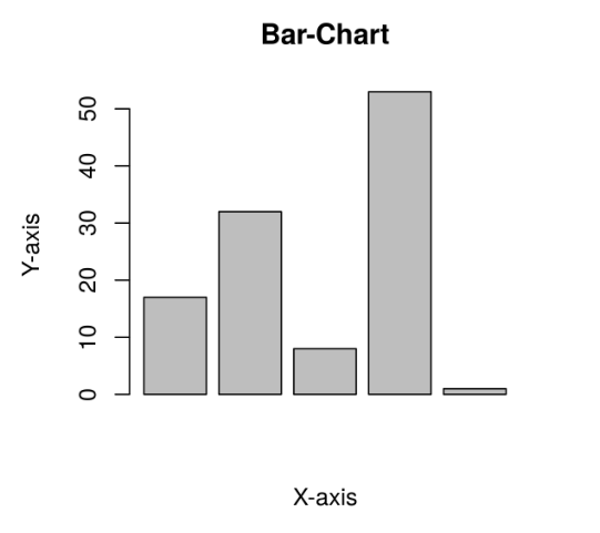
Note: For more information, refer Bar Charts in R
Histograms:
R creates histogram using hist() function.
Example:
R
v <- c(19, 23, 11, 5, 16, 21, 32,
14, 19, 27, 39)
hist(v, xlab = "No.of Articles ",
col = "green", border = "black")
|
Output:

Note: For more information, refer Histograms in R language
Scatter plots:
The simple scatterplot is created using the plot() function.
Example:
R
A <- c(17, 32, 8, 53, 1)
B <- c(12, 43, 17, 43, 10)
plot(x=A, y=B, xlab = "X-axis", ylab = "Y-axis",
main ="Scatter Plot")
|
Output:

Note: For more information, refer Scatter plots in R Language
Line Chart:
The plot() function in R is used to create the line graph.
Example:
R
v <- c(17, 25, 38, 13, 41)
plot(v, type = "l", xlab = "X-axis", ylab = "Y-axis",
main ="Line-Chart")
|
Output:

Note: For more information, refer Line Graphs in R Language.
Pie Charts:
R uses the function pie() to create pie charts. It takes positive numbers as a vector input.
Example:
R
geeks<- c(23, 56, 20, 63)
labels <- c("Mumbai", "Pune", "Chennai", "Bangalore")
pie(geeks, labels)
|
Output:

Note: For more information, refer Pie Charts in R Language
Boxplots:
Boxplots are created in R by using the boxplot() function.
R
input <- mtcars[, c('mpg', 'cyl')]
boxplot(mpg ~ cyl, data = mtcars,
xlab = "Number of Cylinders",
ylab = "Miles Per Gallon",
main = "Mileage Data")
|
Output:

Note: For more information, refer Boxplots in R Language
For more articles refer Data Visualization using R
Statistics
Statistics simply means numerical data, and is field of math that generally deals with collection of data, tabulation, and interpretation of numerical data. It is an area of applied mathematics concern with data collection analysis, interpretation, and presentation. Statistics deals with how data can be used to solve complex problems.
Mean, Median and Mode:
- Mean: It is the sum of observation divided by the total number of observations.
- Median: It is the middle value of the data set.
- Mode: It is the value that has the highest frequency in the given data set. R does not have a standard in-built function to calculate mode.
Example:
R
A <- c(17, 12, 8, 53, 1, 12,
43, 17, 43, 10)
print(mean(A))
print(median(A))
mode <- function(x) {
a <- unique(x)
a[which.max(tabulate(match(x, a)))]
}
print(mode(A)
|
Output:
[1] 21.6
[1] 14.5
[1] 17
Note: For more information, refer Mean, Median and Mode in R Programming
Normal Distribution:
Normal Distribution tells about how the data values are distributed. For example, the height of the population, shoe size, IQ level, rolling a dice, and many more. In R, there are 4 built-in functions to generate normal distribution:
- dnorm() function in R programming measures density function of distribution.
dnorm(x, mean, sd)
- pnorm() function is the cumulative distribution function which measures the probability that a random number X takes a value less than or equal to x
pnorm(x, mean, sd)
- qnorm() function is the inverse of pnorm() function. It takes the probability value and gives output which corresponds to the probability value.
qnorm(p, mean, sd)
- rnorm() function in R programming is used to generate a vector of random numbers which are normally distributed.
rnorm(n, mean, sd)
Example:
R
x <- seq(-10, 10, by=0.1)
y = dnorm(x, mean(x), sd(x))
plot(x, y, main='dnorm')
y <- pnorm(x, mean(x), sd(x))
plot(x, y, main='pnorm')
y <- qnorm(x, mean(x), sd(x))
plot(x, y, main='qnorm')
x <- rnorm(x, mean(x), sd(x))
hist(x, breaks=50, main='rnorm')
|
Output:


Note: For more information refer Normal Distribution in R
Binomial Distribution in R Programming:
The binomial distribution is a discrete distribution and has only two outcomes i.e. success or failure. For example, determining whether a particular lottery ticket has won or not, whether a drug is able to cure a person or not, it can be used to determine the number of heads or tails in a finite number of tosses, for analyzing the outcome of a die, etc. We have four functions for handling binomial distribution in R namely:
dbinom(k, n, p)
pbinom(k, n, p)
where n is total number of trials, p is probability of success, k is the value at which the probability has to be found out.
qbinom(P, n, p)
Where P is the probability, n is the total number of trials and p is the probability of success.
rbinom(n, N, p)
Where n is numbers of observations, N is the total number of trials, p is the probability of success.
Example:
R
probabilities <- dbinom(x = c(0:10), size = 10, prob = 1 / 6)
plot(0:10, probabilities, type = "l", main='dbinom')
probabilities <- pbinom(0:10, size = 10, prob = 1 / 6)
plot(0:10, , type = "l", main='pbinom')
x <- seq(0, 1, by = 0.1)
y <- qbinom(x, size = 13, prob = 1 / 6)
plot(x, y, type = 'l')
probabilities <- rbinom(8, size = 13, prob = 1 / 6)
hist(probabilities)
|
Output:


Note: For more information, refer Binomial Distribution in R Programming
Time Series Analysis:
Time Series in R is used to see how an object behaves over a period of time. In R, it can be easily done by ts() function.
Example: Let’s take the example of COVID-19 pandemic situation. Taking total number of positive cases of COVID-19 cases weekly from 22 January, 2020 to 15 April, 2020 of the world in data vector.
R
x <- c(580, 7813, 28266, 59287, 75700,
87820, 95314, 126214, 218843, 471497,
936851, 1508725, 2072113)
library(lubridate)
mts <- ts(x, start = decimal_date(ymd("2020-01-22")),
frequency = 365.25 / 7)
plot(mts, xlab ="Weekly Data",
ylab ="Total Positive Cases",
main ="COVID-19 Pandemic",
col.main ="darkgreen")
|
Output:
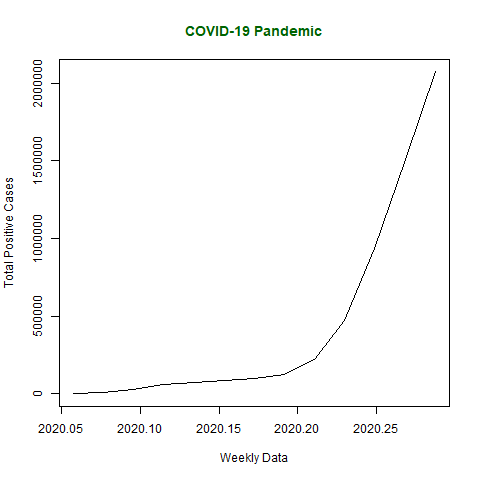
Note: For more information, refer Time Series Analysis in R
Like Article
Suggest improvement
Share your thoughts in the comments
Please Login to comment...