Kolmogorov-Smirnov Test in R Programming

The Kolmogorov-Smirnov Test is a type of non-parametric test of the equality of discontinuous and continuous of a 1D probability distribution that is used to compare the sample with the reference probability test (known as one-sample K-S Test) or among two samples (known as two-sample K-S test). A K-S Test quantifies a distance between the cumulative distribution function of the given reference distribution and the empirical distributions of given two samples, or between the empirical distribution of given two samples. In a one-sample K-S test, the distribution that is considered under a null hypothesis can be purely discrete or continuous or mixed. In the two-sample K-S test, the distribution considered under the null hypothesis is generally continuous distribution but it is unrestricted otherwise. The Kolmogorov-Smirnov test can be done very easily in R Programming.

Kolmogorov-Smirnov Test Formula

The formula for the Kolmogorov-Smirnov test can be given as:

where,

sup_x : the supremum of the set of distances

F_n(x) : the empirical distribution function for n id observations X_i

The empirical distribution function is a distribution function that is associated with the empirical measures of the chosen sample. Being a step function, this cumulative distribution jumps up by a 1/n step at each and every n data points. 

Implementation in R

The K-S test can be performed using the ks.test() function in R. 

Syntax:

ks.text(x, y, …, alternative = c(“two.sided”, “less”, “greater”), exact= NULL, tol= 1e-8, 
simulate.p.value = FALSE, B=2000)

Parameters:

x: numeric vector of data values
y: numeric vector of data values or a character string which is used to name a cumulative distribution function.
…: the parameters which are defined by the y value

alternative: used to indicate the alternate hypothesis.
exact: usually NULL or it indicates a logic that an exact p-value should be computed.

tol: an upper bound used for rounding off errors in the data values.
simulate.p.value: a logic that checks whether to use Monte Carlo method to compute the p-value.
B: an integer value that indicates the number of replicates to be created while using the Monte Carlo method.

Let us understand how to execute a K-S Test step by step using an example of a two-sample K-S test. 

• Step 1: At first install the required packages. For performing the K-S test we need to install the “dgof” package using the install.packages() function from the R console.

install.packages("dgof")

• Step 2: After a successful installation of the package, load the required package in our R Script. for that purpose, use the library() function as follows:

R

# loading the required package
library("dgof")

• Step 3: Use the rnorm() function and the runif() function to generate to samples say x and y. The rnorm() function is used to generate random variates while the runif() function is used to generate random deviates.

R

# loading the required package
library(dgof)

# generating random variate
# sample 1
x <- rnorm(50)

# generating random deviates
# sample 2
y <- runif(30)

• Step 4: Now perform the K-S test on these two samples. For that purpose, use the ks.test() of the dgof package.

R

# loading the required package
library(dgof)

# generating random variate
# sample 1
x <- rnorm(50)

# generating random deviates
# sample 2
y <- runif(30)

# performing the K-S Test
# Do x and y come from
# the same distribution?
ks.test(x, y)

Output:

    Two-sample Kolmogorov-Smirnov test

data:  x and y
D = 0.84, p-value = 5.151e-14
alternative hypothesis: two-sided

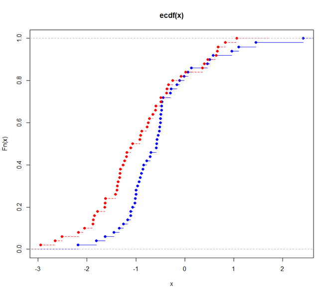
Visualization of the Kolmogorov- Smirnov Test in R

Being quite sensitive to the difference of shape and location of the empirical cumulative distribution of the chosen two samples, the two-sample K-S test is efficient, and one of the most general and useful non-parametric test. Hence we will see how the graph represents the difference between the two samples.

Example:

Here we are generating both the samples using the rnorm() functions and then plot them.  

R

# loading the required package
library(dgof)

# sample 1
# generating a random variate
x <- rnorm(50)

# sample 2
# generating a random variate
x2 <- rnorm(50, -1)

# plotting the result
# visualization
plot(ecdf(x),
     xlim = range(c(x, x2)),
     col = "blue")
plot(ecdf(x2),
     add = TRUE,
     lty = "dashed",
     col = "red")

# performing the K-S
# Test on x and x2
ks.test(x, x2, alternative = "l")

Output:

    Two-sample Kolmogorov-Smirnov test

data:  x and x2
D^- = 0.34, p-value = 0.003089
alternative hypothesis: the CDF of x lies below that of y