Inverse Gamma Distribution in Python

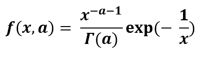
Inverse Gamma distribution is a continuous probability distribution with two parameters on the positive real line. It is the reciprocate distribution of a variable distributed according to the gamma distribution. It is very useful in Bayesian statistics as the marginal distribution for the unknown variance of a normal distribution. It is used for considering the alternate parameter for the normal distribution in terms of the precision which is actually the reciprocal of the variance.

scipy.stats.invgamma() :

It is an inverted gamma continuous random variable. It is an instance of the rv_continuous class. It inherits from the collection of generic methods and combines them with the complete specification of distribution.

Code #1 : Creating inverted gamma continuous random variable

from scipy.stats import invgamma

numargs = invgamma.numargs
[a] = [0.3] * numargs
rv = invgamma (a)

print ("RV : \n", rv)

Output :

RV :
scipy.stats._distn_infrastructure.rv_frozen object at 0x00000230B0B28748

Code #2 : Inverse Gamma continuous variates and probability distribution

import numpy as np
quantile = np.arange (0.01, 1, 0.1)

# Random Variates
R = invgamma.rvs(a, scale = 2,  size = 10)
print ("Random Variates : \n", R)

# PDF
R = invgamma .pdf(a, quantile, loc = 0, scale = 1)
print ("\nProbability Distribution : \n", R)

Output :

Random Variates : 
 [4.18816252e+00 2.02807957e+03 8.37914946e+01 1.94368997e+00
 3.78345091e+00 1.00496176e+06 3.42396458e+03 3.45520522e+00
 2.81037118e+00 1.72359706e+03]

Probability Distribution : 
 [0.0012104  0.0157619  0.03512042 0.05975504 0.09007126 0.12639944
 0.16898506 0.21798098 0.27344182 0.33532072]

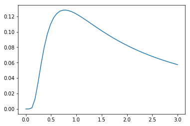
Code #3 : Graphical Representation.

import numpy as np
import matplotlib.pyplot as plt

distribution = np.linspace(0, np.minimum(rv.dist.b, 3))
print("Distribution : \n", distribution)

plot = plt.plot(distribution, rv.pdf(distribution))

Output :

Distribution : 
 [0.         0.06122449 0.12244898 0.18367347 0.24489796 0.30612245
 0.36734694 0.42857143 0.48979592 0.55102041 0.6122449  0.67346939
 0.73469388 0.79591837 0.85714286 0.91836735 0.97959184 1.04081633
 1.10204082 1.16326531 1.2244898  1.28571429 1.34693878 1.40816327
 1.46938776 1.53061224 1.59183673 1.65306122 1.71428571 1.7755102
 1.83673469 1.89795918 1.95918367 2.02040816 2.08163265 2.14285714
 2.20408163 2.26530612 2.32653061 2.3877551  2.44897959 2.51020408
 2.57142857 2.63265306 2.69387755 2.75510204 2.81632653 2.87755102
 2.93877551 3.        ]

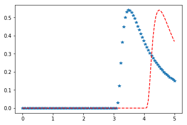
Code #4 : Varying Positional Arguments

import matplotlib.pyplot as plt
import numpy as np

x = np.linspace(0, 5, 100)

# Varying positional arguments
y1 = invgamma .pdf(x, 1, 3)
y2 = invgamma .pdf(x, 1, 4)
plt.plot(x, y1, "*", x, y2, "r--")

Output :