Inventory Demand Forecasting using Machine Learning – Python
Last Updated :
26 Oct, 2022
The vendors who are selling everyday items need to keep their stock up to date so, that no customer returns from their shop empty hand.
Inventory Demand Forecasting using Machine Learning
In this article, we will try to implement a machine learning model which can predict the stock amount for the different products which are sold in different stores.
Importing Libraries and Dataset
Python libraries make it easy for us to handle the data and perform typical and complex tasks with a single line of code.
- Pandas – This library helps to load the data frame in a 2D array format and has multiple functions to perform analysis tasks in one go.
- Numpy – Numpy arrays are very fast and can perform large computations in a very short time.
- Matplotlib/Seaborn – This library is used to draw visualizations.
- Sklearn – This module contains multiple libraries are having pre-implemented functions to perform tasks from data preprocessing to model development and evaluation.
- XGBoost – This contains the eXtreme Gradient Boosting machine learning algorithm which is one of the algorithms which helps us to achieve high accuracy on predictions.
Python3
import numpy as np
import pandas as pd
import matplotlib.pyplot as plt
import seaborn as sb
from sklearn.model_selection import train_test_split
from sklearn.preprocessing import LabelEncoder, StandardScaler
from sklearn import metrics
from sklearn.svm import SVC
from xgboost import XGBRegressor
from sklearn.linear_model import LinearRegression, Lasso, Ridge
from sklearn.ensemble import RandomForestRegressor
from sklearn.metrics import mean_absolute_error as mae
import warnings
warnings.filterwarnings('ignore')
|
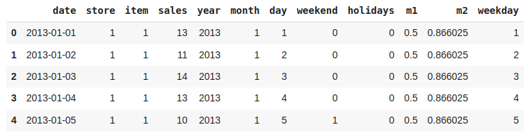
Now let’s load the dataset into the panda’s data frame and print its first five rows.
Python3
df = pd.read_csv('StoreDemand.csv')
display(df.head())
display(df.tail())
|
Output:

First five rows of the dataset.
As we can see we have data for five years for 10 stores and 50 products so, if we calculate it,
(365 * 4 + 366) * 10 * 50 = 913000
Now let’s check the size we have calculated is correct or not .
Output:
(913000, 4)
Let’s check which column of the dataset contains which type of data.
Output:

Information regarding data in the columns
As per the above information regarding the data in each column we can observe that there are no null values.
Output:
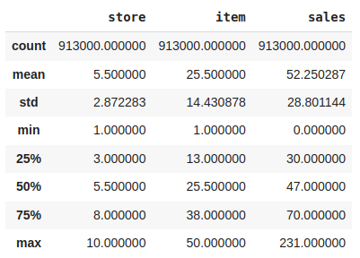
Descriptive statistical measures of the dataset
Feature Engineering
There are times when multiple features are provided in the same feature or we have to derive some features from the existing ones. We will also try to include some extra features in our dataset so, that we can derive some interesting insights from the data we have. Also if the features derived are meaningful then they become a deciding factor in increasing the model’s accuracy significantly.
Python3
parts = df["date"].str.split("-", n = 3, expand = True)
df["year"]= parts[0].astype('int')
df["month"]= parts[1].astype('int')
df["day"]= parts[2].astype('int')
df.head()
|
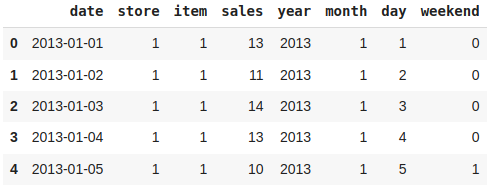
Output:

Addition of day, month, and year feature
Whether it is a weekend or a weekday must have some effect on the requirements to fulfill the demands.
Python3
from datetime import datetime
import calendar
def weekend_or_weekday(year,month,day):
d = datetime(year,month,day)
if d.weekday()>4:
return 1
else:
return 0
df['weekend'] = df.apply(lambda x:weekend_or_weekday(x['year'], x['month'], x['day']), axis=1)
df.head()
|
Output:
Addition of a weekend feature
It would be nice to have a column which can indicate whether there was any holiday on a particular day or not.
Python3
from datetime import date
import holidays
def is_holiday(x):
india_holidays = holidays.country_holidays('IN')
if india_holidays.get(x):
return 1
else:
return 0
df['holidays'] = df['date'].apply(is_holiday)
df.head()
|
Output:
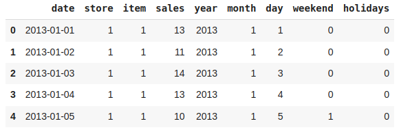
Addition of a holiday feature
Now, let’s add some cyclical features.
Python3
df['m1'] = np.sin(df['month'] * (2 * np.pi / 12))
df['m2'] = np.cos(df['month'] * (2 * np.pi / 12))
df.head()
|
Output:
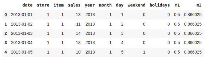
Addition of Cyclical Features
Let’s have a column whose value indicates which day of the week it is.
Python3
def which_day(year, month, day):
d = datetime(year,month,day)
return d.weekday()
df['weekday'] = df.apply(lambda x: which_day(x['year'],
x['month'],
x['day']),
axis=1)
df.head()
|
Output:
Addition of weekday Features
Now let’s remove the columns which are not useful for us.
Python3
df.drop('date', axis=1, inplace=True)
|
There may be some other relevant features as well which can be added to this dataset but let’s try to build a build with these ones and try to extract some insights as well.
Exploratory Data Analysis
EDA is an approach to analyzing the data using visual techniques. It is used to discover trends, and patterns, or to check assumptions with the help of statistical summaries and graphical representations.
We have added some features to our dataset using some assumptions. Now let’s check what are the relations between different features with the target feature.
Python3
df['store'].nunique(), df['item'].nunique()
|
Output:
(10, 50)
From here we can conclude that there are 10 unique stores and they sell 50 different products.
Python3
features = ['store', 'year', 'month',\
'weekday', 'weekend', 'holidays']
plt.subplots(figsize=(20, 10))
for i, col in enumerate(features):
plt.subplot(2, 3, i + 1)
df.groupby(col).mean()['sales'].plot.bar()
plt.show()
|
Output:

Bar plot for the average count of the ride request
Now let’s check the variation of stock as the month closes to the end.
Python3
plt.figure(figsize=(10,5))
df.groupby('day').mean()['sales'].plot()
plt.show()
|
Output:

Line plot for the average count of stock required on the respective days of the month
Let’s draw the simple moving average for 30 days period.
Python3
plt.figure(figsize=(15, 10))
window_size = 30
data = df[df['year']==2013]
windows = data['sales'].rolling(window_size)
sma = windows.mean()
sma = sma[window_size - 1:]
data['sales'].plot()
sma.plot()
plt.legend()
plt.show()
|
Output:
As the data in the sales column is continuous let’s check the distribution of it and check whether there are some outliers in this column or not.
Python3
plt.subplots(figsize=(12, 5))
plt.subplot(1, 2, 1)
sb.distplot(df['sales'])
plt.subplot(1, 2, 2)
sb.boxplot(df['sales'])
plt.show()
|
Output:

Distribution plot and Box plot for the target column
Highly correlated features do
Python3
plt.figure(figsize=(10, 10))
sb.heatmap(df.corr() > 0.8,
annot=True,
cbar=False)
plt.show()
|
Output:
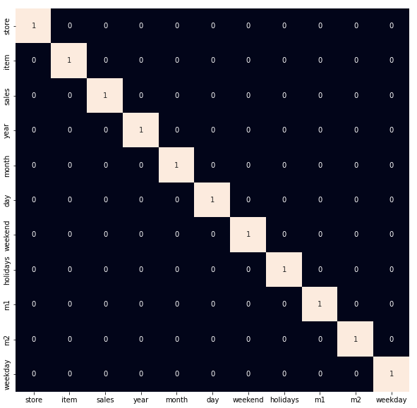
Heatmap to detect the highly correlated features
As we observed earlier let’s remove the outliers which are present in the data.
Model Training
Now we will separate the features and target variables and split them into training and the testing data by using which we will select the model which is performing best on the validation data.
Python3
features = df.drop(['sales', 'year'], axis=1)
target = df['sales'].values
X_train, X_val, Y_train, Y_val = train_test_split(features, target,
test_size = 0.05,
random_state=22)
X_train.shape, X_val.shape
|
Output:
((861170, 9), (45325, 9))
Normalizing the data before feeding it into machine learning models helps us to achieve stable and fast training.
Python3
scaler = StandardScaler()
X_train = scaler.fit_transform(X_train)
X_val = scaler.transform(X_val)
|
We have split our data into training and validation data also the normalization of the data has been done. Now let’s train some state-of-the-art machine learning models and select the best out of them using the validation dataset.
Python3
models = [LinearRegression(), XGBRegressor(), Lasso(), Ridge()]
for i in range(4):
models[i].fit(X_train, Y_train)
print(f'{models[i]} : ')
train_preds = models[i].predict(X_train)
print('Training Error : ', mae(Y_train, train_preds))
val_preds = models[i].predict(X_val)
print('Validation Error : ', mae(Y_val, val_preds))
print()
|
Output:
LinearRegression() :
Training Error :  20.902897365994484
Validation Error :  20.97143554027027

[08:31:23] WARNING: /workspace/src/objective/regression_obj.cu:152:
reg:linear is now deprecated in favor of reg:squarederror.
XGBRegressor() :
Training Error :  11.751541013057603
Validation Error :  11.790298395298885

Lasso() :
Training Error :  21.015028699769758
Validation Error :  21.071517213774968

Ridge() :
Training Error :  20.90289749951532
Validation Error :  20.971435731904066
Like Article
Suggest improvement
Share your thoughts in the comments
Please Login to comment...