What is Adam Optimizer?

Prerequisites :  Optimization techniques in Gradient Descent

Adam Optimizer 

Adaptive Moment Estimation is an algorithm for optimization technique for gradient descent. The method is really efficient when working with large problem involving a lot of data or parameters. It requires less memory and is efficient. Intuitively, it is a combination of the ‘gradient descent with momentum’ algorithm and the ‘RMSP’ algorithm.

How Adam works?

Adam optimizer involves a combination of two gradient descent methodologies: 

Momentum:

This algorithm is used to accelerate the gradient descent algorithm by taking into consideration the ‘exponentially weighted average’ of the gradients. Using averages makes the algorithm converge towards the minima in a faster pace. 

[Tex]w_{t+1}=w_{t}-\alpha m_{t}[/Tex]

where,

[Tex]m_{t}=\beta m_{t-1}+(1-\beta)\left[\frac{\delta L}{\delta w_{t}}\right][/Tex]

m_t = aggregate of gradients at time t [current] (initially, m_t = 0) m_t-1 = aggregate of gradients at time t-1 [previous] W_t = weights at time t W_t+1 = weights at time t+1 α_t = learning rate at time t ∂L = derivative of Loss Function ∂W_t = derivative of weights at time t β = Moving average parameter (const, 0.9)

Root Mean Square Propagation (RMSP): 

Root mean square prop or RMSprop is an adaptive learning algorithm that tries to improve AdaGrad. Instead of taking the cumulative sum of squared gradients like in AdaGrad, it takes the ‘exponential moving average’.

[Tex]w_{t+1}=w_{t}-\frac{\alpha_{t}}{\left(v_{t}+\varepsilon\right)^{1 / 2}} *\left[\frac{\delta L}{\delta w_{t}}\right][/Tex]

where, 

[Tex]v_{t}=\beta v_{t-1}+(1-\beta) *\left[\frac{\delta L}{\delta w_{t}}\right]^{2}[/Tex]

W_t = weights at time t W_t+1 = weights at time t+1 α_t = learning rate at time t ∂L = derivative of Loss Function ∂W_t = derivative of weights at time t V_t = sum of square of past gradients. [i.e sum(∂L/∂Wt-1)] (initially, V_t = 0) β = Moving average parameter (const, 0.9) ϵ = A small positive constant (10^-8)

NOTE: Time (t) could be interpreted as an Iteration (i). 

Adam Optimizer inherits the strengths or the positive attributes of the above two methods and builds upon them to give a more optimized gradient descent. 

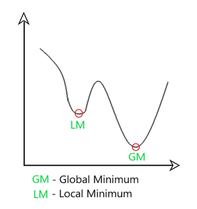
Here, we control the rate of gradient descent in such a way that there is minimum oscillation when it reaches the global minimum while taking big enough steps (step-size) so as to pass the local minima hurdles along the way. Hence, combining the features of the above methods to reach the global minimum efficiently. 

Mathematical Aspect of Adam Optimizer

Taking the formulas used in the above two methods, we get

[Tex]\begin{aligned} m_{t}&=\beta_{1} m_{t-1}+\left(1-\beta_{1}\right)\left[\frac{\delta L}{\delta w_{t}}\right] \\ v_{t}&=\beta_{2} v_{t-1}+\left(1-\beta_{2}\right)\left[\frac{\delta L}{\delta w_{t}}\right]^{2} \end{aligned}[/Tex]

Parameters Used : 1. ϵ = a small +ve constant to avoid 'division by 0' error when (v_t -> 0). (10^-8) 2. β₁ & β₂ = decay rates of average of gradients in the above two methods. (β₁ = 0.9 & β₂ = 0.999) 3. α — Step size parameter / learning rate (0.001)

Since m_t and v_t have both initialized as 0 (based on the above methods), it is observed that they gain a tendency to be ‘biased towards 0’ as both β₁ & β₂ ≈ 1. This Optimizer fixes this problem by computing ‘bias-corrected’ m_t and v_t. This is also done to control the weights while reaching the global minimum to prevent high oscillations when near it. The formulas used are:

[Tex]\widehat{m_{t}}=\frac{m_{t}}{1-\beta_{1}^{t}} \widehat{v}_{t}=\frac{v_{t}}{1-\beta_{2}^{t}}[/Tex]

Intuitively, we are adapting to the gradient descent after every iteration so that it remains controlled and unbiased throughout the process, hence the name Adam. 

Now, instead of our normal weight parameters m_t and v_t , we take the bias-corrected weight parameters (m_hat)_t and (v_hat)_t. Putting them into our general equation, we get

[Tex]w_{t+1}=w_{t}-\widehat{m_{t}}\left(\frac{\alpha}{\sqrt{\widehat{v_{t}}}+\varepsilon}\right)[/Tex]

Performance:

Building upon the strengths of previous models, Adam optimizer gives much higher performance than the previously used and outperforms them by a big margin into giving an optimized gradient descent. The plot is shown below clearly depicts how Adam Optimizer outperforms the rest of the optimizer by a considerable margin in terms of training cost (low) and performance (high). 

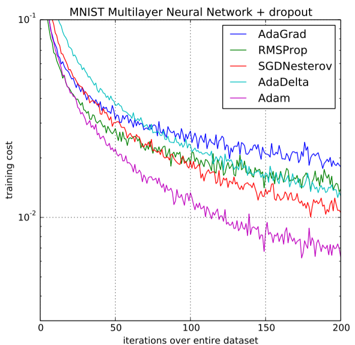
Performance Comparison on Training cost