Introductory guide to Information Retrieval using KNN and KDTree

What is Information Retrieval(IR)?

It can be defined as a software program that is used to find material(usually documents) of an unstructured nature(usually text) that satisfies an information need from within large collections(usually stored on computers). It helps users find their required information but does not explicitly return the answers to their questions. It gives information about the existence and location of the documents that might contain the required information.

Use Cases of Information Retrieval

Information Retrieval can be used in many scenarios, some of these are:

• Web Search
• E-mail Search
• Searching your laptop
• Legal information retrieval etc.

Process of Information Retrieval

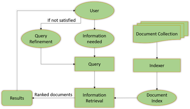
To learn more about information retrieval you can refer to this article.

Here we are going to discuss two algorithms that are used in Information Retrieval:

1. K-Nearest Neighbors(KNN)
2. K-Dimensional Tree(KDTree)

K-Nearest Neighbor (KNN)

It is a supervised machine-learning classification algorithm. Classification gives information regarding what group something belongs to, for example, the type of tumor, the favorite sport of a person, etc. The K in KNN stands for the number of the nearest neighbors that the classifier will use to make its prediction.

We have training data with which we can predict the query data. For the query record which needs to be classified, the KNN algorithm computes the distance between the query record and all of the training data records. Then it looks at the K closest data records in the training data.

How to choose the K value?

While choosing the K value, keep following these things in mind:

• If K=1, the classes are divided into regions and the query record belongs to a class according to the region it lies in.
• Choose odd values of K for a 2-class problem.
• K must not be a multiple of the number of classes. K is not equal to ‘ni’, where n is the number of classes and i = 1, 2, 3….

Distance Metrics: The different distance metrics which can be used are:

• Euclidean Distance
• Manhattan Distance
• Hamming Distance
• Minkowski Distance
• Chebyshev Distance

Let’s take an example to understand in detail how the KNN algorithm works. Given below is a small dataset to predict which Pizza outlet a person prefers out of Pizza Hut & Dominoes.

NAME	AGE	CHEESE CONTENT	PIZZA OUTLET
Riya	30	6.2	Pizza Hut
Manish	15	8	Dominos
Rachel	42	4	Pizza Hut
Rahul	20	8.4	Pizza Hut
Varun	54	3.3	Dominos
Mark	47	5	Pizza Hut
Sakshi	27	9	Dominos
David	17	7	Dominos
Arpita	8	9.2	Pizza Hut
Ananya	35	7.6	Dominos

The outlet is chosen on the basis of the Age of the person and how much Cheese Content the person like(on a scale of 10).

This data can be visualized graphically as: 

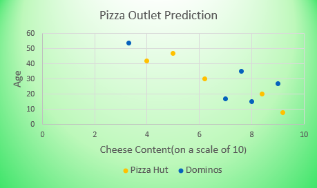
Note: If we have discrete data we first have to convert it into numeric data. Ex: Gender is given as Male and Female we can convert it to numeric as 0 and 1.

• Since we have 2 classes — Pizza Hut and Domino, we’ll take K=3.
• To calculate the distance we are using the Euclidean Distance –

Prediction: On the basis of the above data we need to find out the result for the query:

NAME	AGE	CHEESE CONTENT	PIZZA OUTLET
Harry	46	7	???

• Now find the distance of the record Harry to all the other records.

         Given below is the calculation for the distance from Harry to Riya:

        Similarly, the Distances from all the records are:

NAME	PIZZA OUTLET	DISTANCE
Riya	Pizza Hut	16.01
Manish	Dominos	31.01
Rachel	Pizza Hut	5
Rahul	Pizza Hut	26.03
Varun	Dominos	8.81
Mark	Pizza Hut	2.23
Sakshi	Dominos	19.10
David	Dominos	29
Arpita	Pizza Hut	38.06
Ananya	Dominos	11.01

From the table, we can see that the K(3) closest distances are of Mark, Rachel, and Varun, and Pizza Outlet they prefer are Pizza Hut, Pizza Hut, and Domino respectively. Hence, we can make the prediction that Harry prefers Pizza Hut.

Advantages of using the KNN Algorithm: 

• No training phase
• It can learn complex models easily
• It is robust to noisy training data

Disadvantages of using the KNN Algorithm: 

• Determining the value of parameter K can be difficult as different K values can give different results.
• It is hard to apply on High Dimensional data
• Computation cost is high as each query it has to go through all the records which takes O(N) time, where N is the number of records. If we maintain a priority queue to return the closest K records then the time complexity will be O(log(K)*N).

Due to the high computational cost, we use an algorithm that is time efficient and similar in approach – KDTree Algorithm.

K-Dimensional Tree (KDTree)

KDTree is a space partitioning data structure for organizing points in K-Dimensional space. It is an improvement over KNN. It is useful for representing data efficiently. In KDTree the data points are organized and partitioned on the basis of some specific conditions.

How the algorithm works:

To understand this let’s take the sample data of Pizza Outlet which we considered in the previous example. Basically, we make some axis-aligned cuts and create different regions, keeping the track of points that lie in these regions. Each region is represented by a node in the tree.

• Split the regions at the mean value of the observations.

For the first cut, we’ll find the mean of all the X-coordinates (Cheese Content in this case).

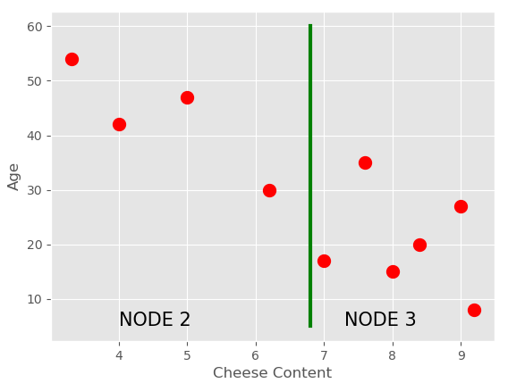
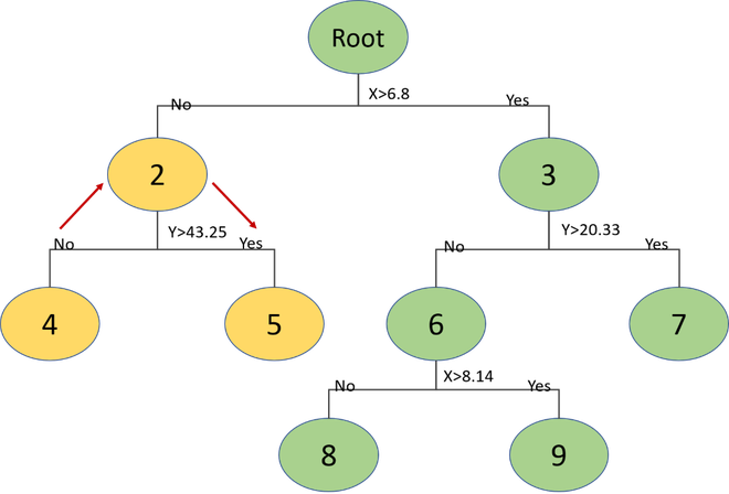
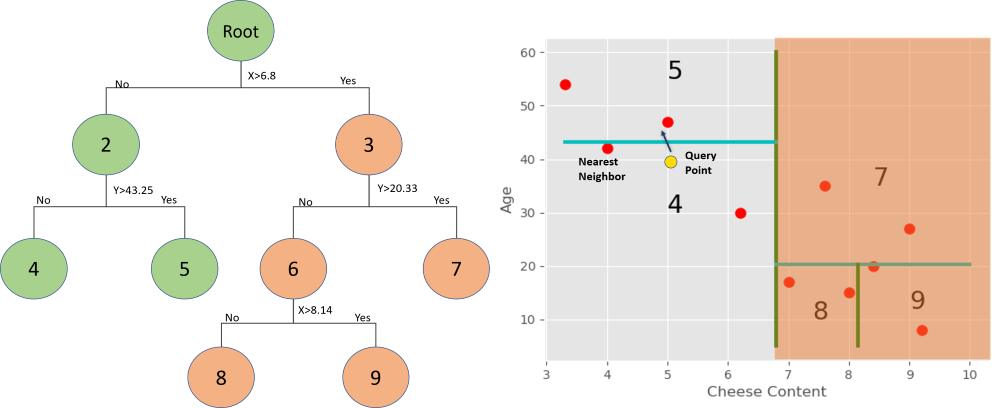
Now on both regions, we’ll calculate the means of Y-coordinates to make the cuts and so on, repeating the steps until the number of points in each region is less than a given number. You can choose any number less than the number of records in the dataset otherwise we’ll have only 1 region. The complete tree structure for this will be:

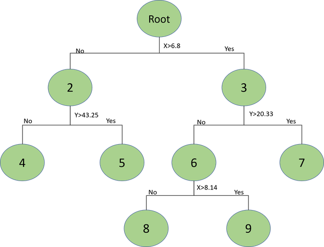
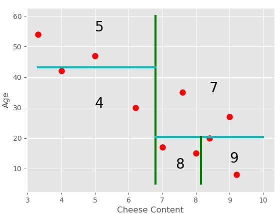
Here there are fewer than 3 points in each region.

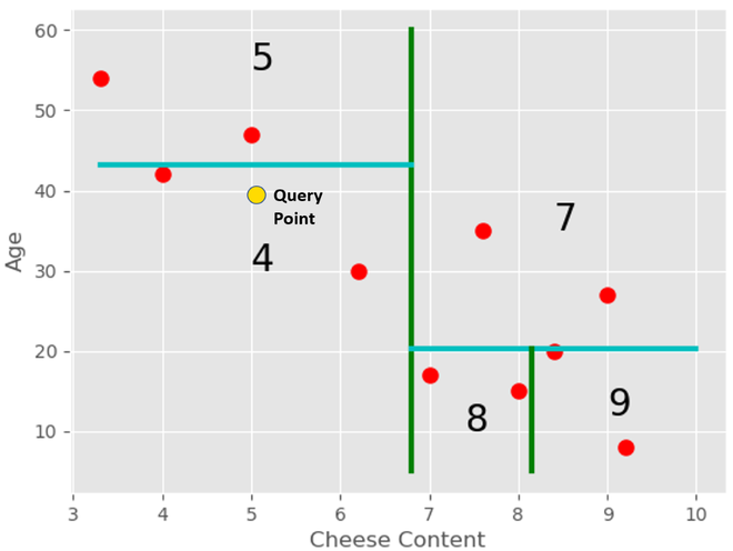
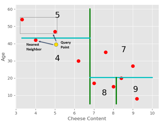
Now if a new query point comes, and we need to find out in which region will the point be, we can traverse the tree. In this case, the query point(chosen randomly) lies in the 4th region.

We can find it’s the nearest neighbor in this region.

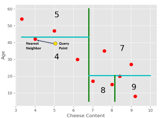
But this might not be the actual nearest neighbor for this query in the entire dataset. Hence we traverse back to node 2 and then check the remaining subtree for this node.

We get the tightest box for node 5 which contains all the points in this region. After that, we check if the distance of this box is closer to the query point than the current nearest neighbor or not.

In this case, the distance of the box is smaller. Hence, there is a point in the region point which is closer to the query point than the current nearest neighbor. We find that point, and then we again traverse back the tree to node 3 and check the same.

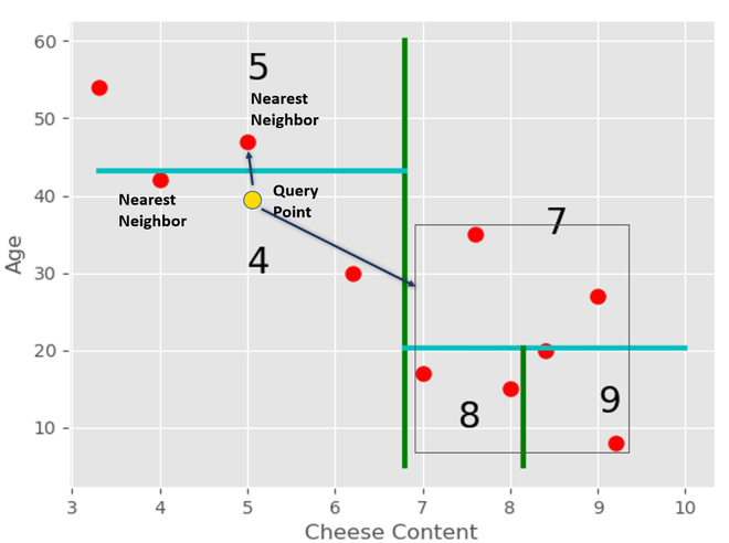
Now the distance is greater than the distance from the new nearest neighbor. Hence, we stop here, and we do not need to search for this sub-tree. We can prune this part of the tree.

Note: A branch of the tree is eliminated only when K points have been found and the branch cannot have points closer than any of the K current bests.

KD tree Implementation: 

We will be performing Document Retrieval which is the most widely used use case for Information Retrieval. For this, we have made a sample dataset of articles available on the internet on famous celebrities. On entering the name you get the names of the celebrities similar to the given name. Here the K value is taken as 3. We will get the three nearest neighbors of the document name entered.

You can get the dataset from here.

Code: 

python3

#import the libraries required
import numpy as np
import pandas as pd
import nltk
from sklearn.feature_extraction.text import CountVectorizer, TfidfTransformer
from sklearn.neighbors import KDTree

#Reading the dataset
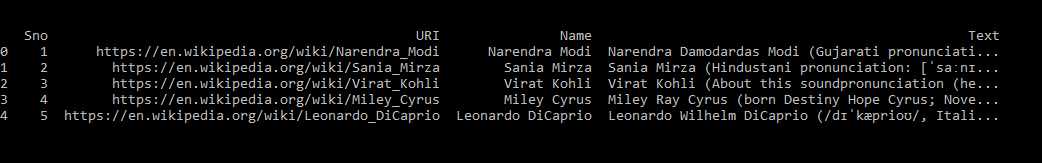
person = pd.read_csv('famous_people.csv')

#Printing first five rows of the dataset
print(person.head())

Output:

Code: 

python3

#Counting the frequency of occurrence of each word
count_vector = CountVectorizer()
train_counts = count_vector.fit_transform(person.Text)

#Using tf-idf to reduce the weight of common words
tfidf_transform = TfidfTransformer()
train_tfidf = tfidf_transform.fit_transform(train_counts)
a = np.array(train_tfidf.toarray())

#obtaining the KDTree
kdtree = KDTree(a ,leaf_size=3)

#take the name of the personality as input
person_name=input("Enter the name of the Person:- ")

#Using KDTree to get K articles similar to the given name
person['tfidf']=list(train_tfidf.toarray())
distance, idx = kdtree.query(person['tfidf'][person['Name']== person_name].tolist(), k=3)
for i, value in list(enumerate(idx[0])):
    print("Name : {}".format(person['Name'][value]))
    print("Distance : {}".format(distance[0][i]))
    print("URI : {}".format(person['URI'][value]))

Output:

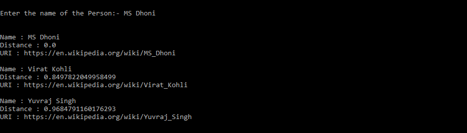
We get MS Dhoni, Virat Kohli, and Yuvraj Singh as the 3 nearest neighbors for MS Dhoni.

Advantages of using KDTree

• At each level of the tree, KDTree divides the range of the domain in half. Hence they are useful for performing range searches.
• It is an improvement of KNN as discussed earlier.
• The complexity lies in between O(log N) to O(N) where N is the number of nodes in the tree.

Disadvantages of using KDTree

• Degradation of performance when high dimensional data is used. The algorithm will need to visit many more branches. If the dimensionality of a dataset is K then the number of nodes N>>(2^K).
• If the query point is far from all the points in the dataset then we might have to traverse the whole tree to find the nearest neighbors.

For any queries do leave a comment below.