Introduction to Sorting Techniques – Data Structure and Algorithm Tutorials

Last Updated : 30 Mar, 2023

Sorting refers to rearrangement of a given array or list of elements according to a comparison operator on the elements. The comparison operator is used to decide the new order of elements in the respective data structure.

When we have a large amount of data, it can be difficult to deal with it, especially when it is arranged randomly. When this happens, sorting that data becomes crucial. It is necessary to sort data in order to make searching easier.

Types of Sorting Techniques

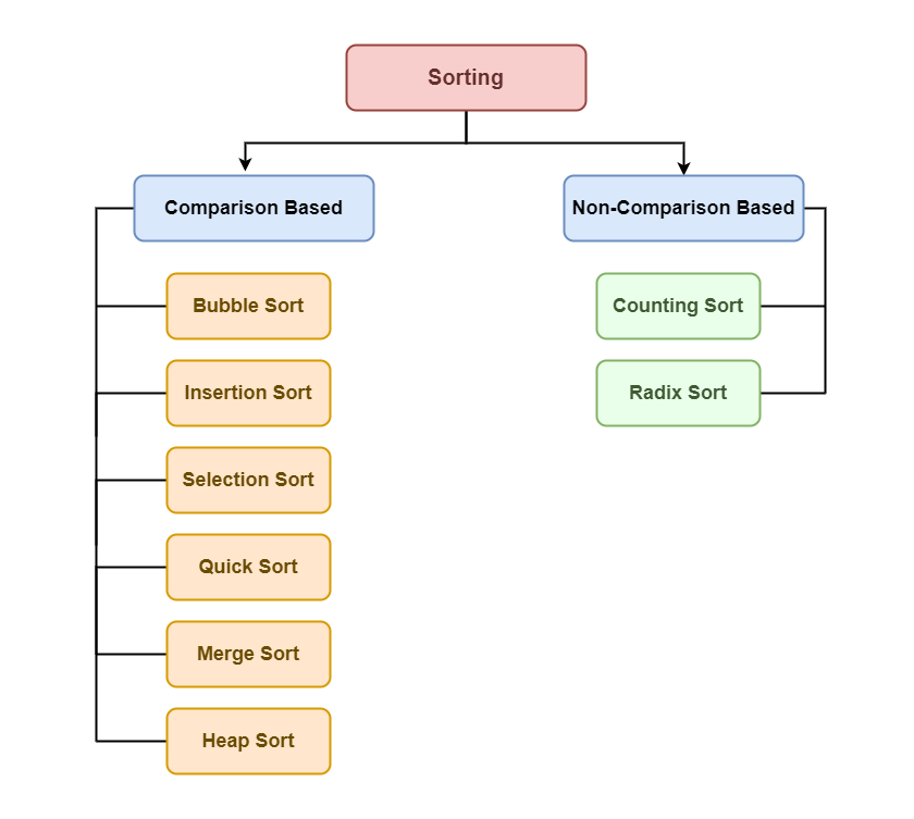
There are various sorting algorithms are used in data structures. The following two types of sorting algorithms can be broadly classified:

Comparison-based: We compare the elements in a comparison-based sorting algorithm)
Non-comparison-based: We do not compare the elements in a non-comparison-based sorting algorithm)

Sorting algorithm

Why Sorting Algorithms are Important

The sorting algorithm is important in Computer Science because it reduces the complexity of a problem. There is a wide range of applications for these algorithms, including searching algorithms, database algorithms, divide and conquer methods, and data structure algorithms.

In the following sections, we list some important scientific applications where sorting algorithms are used

When you have hundreds of datasets you want to print, you might want to arrange them in some way.
Sorting algorithm is used to arrange the elements of a list in a certain order (either ascending or descending).
Searching any element in a huge data set becomes easy. We can use Binary search method for search if we have sorted data. So, Sorting become important here.
They can be used in software and in conceptual problems to solve more advanced problems.

Some of the most common sorting algorithms are:

Below are some of the most common sorting algorithms:

1. Selection sort

Selection sort is another sorting technique in which we find the minimum element in every iteration and place it in the array beginning from the first index. Thus, a selection sort also gets divided into a sorted and unsorted subarray.

Working of Selection Sort algorithm:

Lets consider the following array as an example: arr[] = {64, 25, 12, 22, 11}

First pass:

For the first position in the sorted array, the whole array is traversed from index 0 to 4 sequentially. The first position where 64 is stored presently, after traversing whole array it is clear that 11 is the lowest value.

64    25    12    22    11

Thus, replace 64 with 11. After one iteration 11, which happens to be the least value in the array, tends to appear in the first position of the sorted list.

11    25    12    22    64

Second Pass:

For the second position, where 25 is present, again traverse the rest of the array in a sequential manner.

11    25    12    22    64

After traversing, we found that 12 is the second lowest value in the array and it should appear at the second place in the array, thus swap these values.

11    12    25    22    64

Third Pass:

Now, for third place, where 25 is present again traverse the rest of the array and find the third least value present in the array.

11    12    25    22    64

While traversing, 22 came out to be the third least value and it should appear at the third place in the array, thus swap 22 with element present at third position.

11    12    22    25    64

Fourth pass:

Similarly, for fourth position traverse the rest of the array and find the fourth least element in the array
As 25 is the 4th lowest value hence, it will place at the fourth position.

11    12    22    25    64

Fifth Pass:

At last the largest value present in the array automatically get placed at the last position in the array
The resulted array is the sorted array.

11    12    22    25    64

2. Bubble sort

Bubble Sort is the simplest sorting algorithm that works by repeatedly swapping the adjacent elements if they are in the wrong order. This algorithm is not suitable for large data sets as its average and worst-case time complexity is quite high.

Working of Bubble Sort algorithm:

Lets consider the following array as an example: arr[] = {5, 1, 4, 2, 8}

First Pass:

Bubble sort starts with very first two elements, comparing them to check which one is greater.
( 5 1 4 2 8 ) –> ( 1 5 4 2 8 ), Here, algorithm compares the first two elements, and swaps since 5 > 1.
( 1 5 4 2 8 ) –> ( 1 4 5 2 8 ), Swap since 5 > 4
( 1 4 5 2 8 ) –> ( 1 4 2 5 8 ), Swap since 5 > 2
( 1 4 2 5 8 ) –> ( 1 4 2 5 8 ), Now, since these elements are already in order (8 > 5), algorithm does not swap them.

Second Pass:

Now, during second iteration it should look like this:

( 1 4 2 5 8 ) –> ( 1 4 2 5 8 )
( 1 4 2 5 8 ) –> ( 1 2 4 5 8 ), Swap since 4 > 2
( 1 2 4 5 8 ) –> ( 1 2 4 5 8 )
( 1 2 4 5 8 ) –> ( 1 2 4 5 8 )
Third Pass:

Now, the array is already sorted, but our algorithm does not know if it is completed.
The algorithm needs one whole pass without any swap to know it is sorted.

( 1 2 4 5 8 ) –> ( 1 2 4 5 8 )
( 1 2 4 5 8 ) –> ( 1 2 4 5 8 )
( 1 2 4 5 8 ) –> ( 1 2 4 5 8 )
( 1 2 4 5 8 ) –> ( 1 2 4 5 8 )

Illustration:

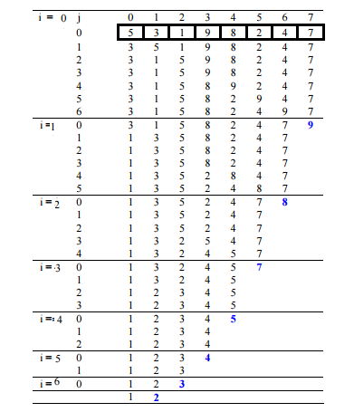
Illustration of Bubble Sort

3. Insertion Sort

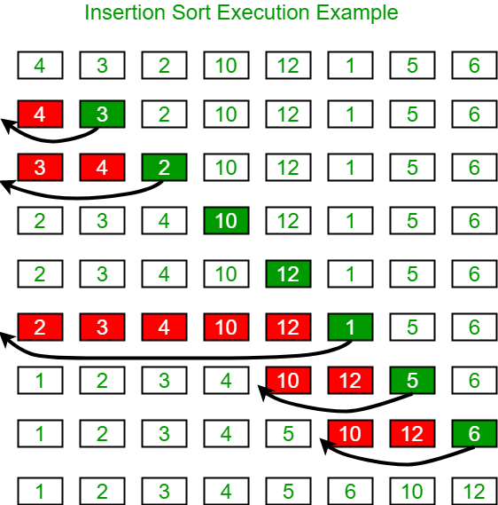
Insertion sort is a simple sorting algorithm that works similarly to the way you sort playing cards in your hands. The array is virtually split into a sorted and an unsorted part. Values from the unsorted part are picked and placed at the correct position in the sorted part.

Working of Insertion Sort algorithm:

Consider an example: arr[]: {12, 11, 13, 5, 6}

12    11    13    5    6

First Pass:

Initially, the first two elements of the array are compared in insertion sort.
12    11    13    5    6
Here, 12 is greater than 11 hence they are not in the ascending order and 12 is not at its correct position. Thus, swap 11 and 12.
So, for now 11 is stored in a sorted sub-array.
11    12    13    5    6

Second Pass:

Now, move to the next two elements and compare them
11    12    13    5    6
Here, 13 is greater than 12, thus both elements seems to be in ascending order, hence, no swapping will occur. 12 also stored in a sorted sub-array along with 11

Third Pass:

Now, two elements are present in the sorted sub-array which are 11 and 12
Moving forward to the next two elements which are 13 and 5
11    12    13    5    6
Both 5 and 13 are not present at their correct place so swap them
11    12    5    13    6
After swapping, elements 12 and 5 are not sorted, thus swap again
11    5    12    13    6
Here, again 11 and 5 are not sorted, hence swap again
5    11    12    13    6
here, it is at its correct position

Fourth Pass:

Now, the elements which are present in the sorted sub-array are 5, 11 and 12
Moving to the next two elements 13 and 6
5    11    12    13    6
Clearly, they are not sorted, thus perform swap between both
5    11    12    6    13
Now, 6 is smaller than 12, hence, swap again
5    11    6    12    13
Here, also swapping makes 11 and 6 unsorted hence, swap again
5    6    11    12    13
Finally, the array is completely sorted.

Illustrations:

4. Merge Sort

The Merge Sort algorithm is a sorting algorithm that is based on the Divide and Conquers paradigm. In this algorithm, the array is initially divided into two equal halves and then they are combined in a sorted manner.

Let’s see how Merge Sort uses Divide and Conquer:

The merge sort algorithm is an implementation of the divide and conquers technique. Thus, it gets completed in three steps:

Divide: In this step, the array/list divides itself recursively into sub-arrays until the base case is reached.
Conquer: Here, the sub-arrays are sorted using recursion.
Combine: This step makes use of the merge( ) function to combine the sub-arrays into the final sorted array.

Working of Merge Sort algorithm:

To know the functioning of merge sort, lets consider an array arr[] = {38, 27, 43, 3, 9, 82, 10}

At first, check if the left index of array is less than the right index, if yes then calculate its mid point

Now, as we already know that merge sort first divides the whole array iteratively into equal halves, unless the atomic values are achieved.
Here, we see that an array of 7 items is divided into two arrays of size 4 and 3 respectively.

Now, again find that is left index is less than the right index for both arrays, if found yes, then again calculate mid points for both the arrays.

Now, further divide these two arrays into further halves, until the atomic units of the array is reached and further division is not possible.

After dividing the array into smallest units, start merging the elements again based on comparison of size of elements
Firstly, compare the element for each list and then combine them into another list in a sorted manner.

After the final merging, the list looks like this:

5. Quick sort

Quicksort is a sorting algorithm based on the divide and conquer approach where an array is divided into subarrays by selecting a pivot element (element selected from the array).

While dividing the array, the pivot element should be positioned in such a way that elements less than the pivot are kept on the left side, and elements greater than the pivot is on the right side of the pivot.
The left and right subarrays are also divided using the same approach. This process continues until each subarray contains a single element.
At this point, elements are already sorted. Finally, elements are combined to form a sorted array.

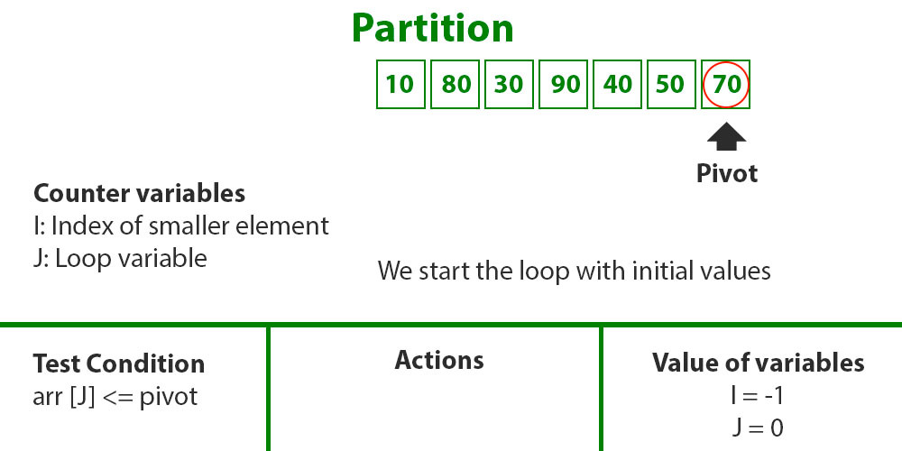
Working of Quick Sort algorithm:

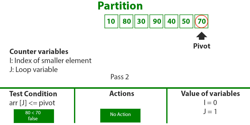
To know the functioning of Quick sort, let’s consider an array arr[] = {10, 80, 30, 90, 40, 50, 70}

Indexes: 0 1 2 3 4 5 6
low = 0, high = 6, pivot = arr[h] = 70
Initialize index of smaller element, i = -1
Step1
Traverse elements from j = low to high-1
j = 0: Since arr[j] <= pivot, do i++ and swap(arr[i], arr[j])
i = 0
arr[] = {10, 80, 30, 90, 40, 50, 70} // No change as i and j are same
j = 1: Since arr[j] > pivot, do nothing
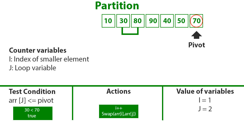
Step2
j = 2 : Since arr[j] <= pivot, do i++ and swap(arr[i], arr[j])
i = 1
arr[] = {10, 30, 80, 90, 40, 50, 70} // We swap 80 and 30
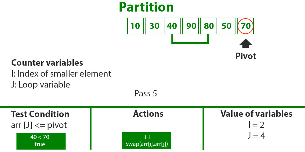
Step3
j = 3 : Since arr[j] > pivot, do nothing // No change in i and arr[]
j = 4 : Since arr[j] <= pivot, do i++ and swap(arr[i], arr[j])
i = 2
arr[] = {10, 30, 40, 90, 80, 50, 70} // 80 and 40 Swapped
Step 4
j = 5 : Since arr[j] <= pivot, do i++ and swap arr[i] with arr[j]
i = 3
arr[] = {10, 30, 40, 50, 80, 90, 70} // 90 and 50 Swapped
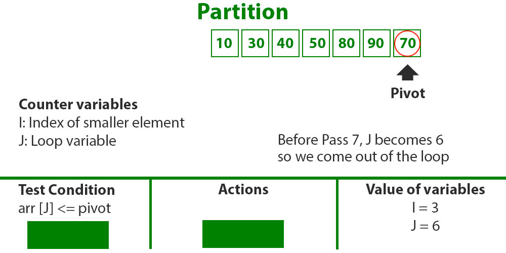
Step 5
We come out of loop because j is now equal to high-1.
Finally we place pivot at correct position by swapping arr[i+1] and arr[high] (or pivot)
arr[] = {10, 30, 40, 50, 70, 90, 80} // 80 and 70 Swapped
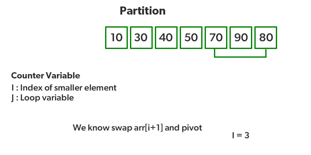
Step 6
Now 70 is at its correct place. All elements smaller than 70 are before it and all elements greater than 70 are after it.
Since quick sort is a recursive function, we call the partition function again at left and right partitions
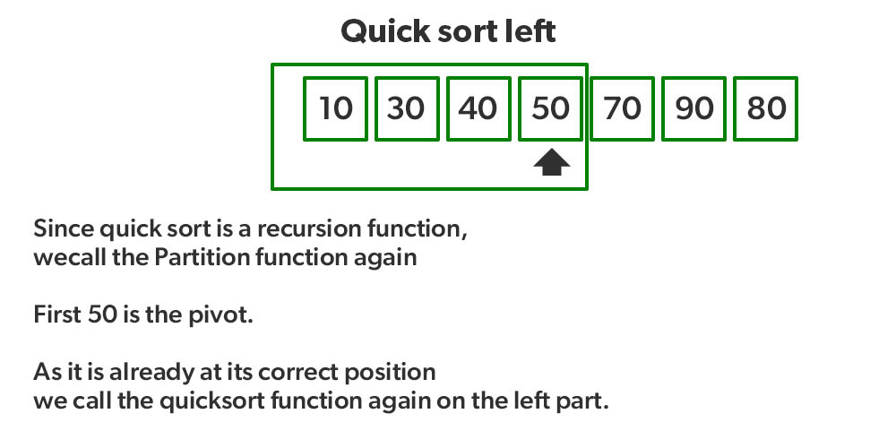
Step 7
Again call function at right part and swap 80 and 90
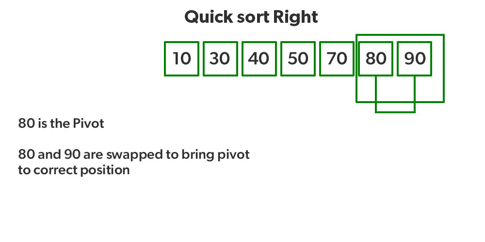
Step 8

6. Heap sort

Heap sort is a comparison-based sorting technique based on Binary Heap data structure. It is similar to the selection sort where we first find the minimum element and place the minimum element at the beginning. Repeat the same process for the remaining elements.

Working of Heap Sort algorithm:

To understand heap sort more clearly, let’s take an unsorted array and try to sort it using heap sort. Consider the array: arr[] = {4, 10, 3, 5, 1}.

Build Complete Binary Tree: Build a complete binary tree from the array.

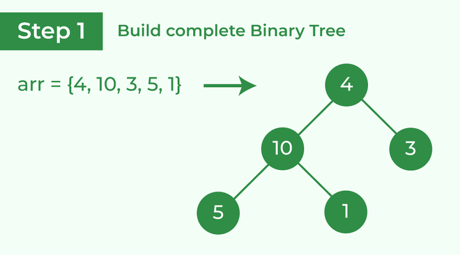
Build complete binary tree from the array

Transform into max heap: After that, the task is to construct a tree from that unsorted array and try to convert it into max heap.

To transform a heap into a max-heap, the parent node should always be greater than or equal to the child nodes
Here, in this example, as the parent node 4 is smaller than the child node 10, thus, swap them to build a max-heap.
Transform it into a max heap

Now, as seen, 4 as a parent is smaller than the child 5, thus swap both of these again and the resulted heap and array should be like this:
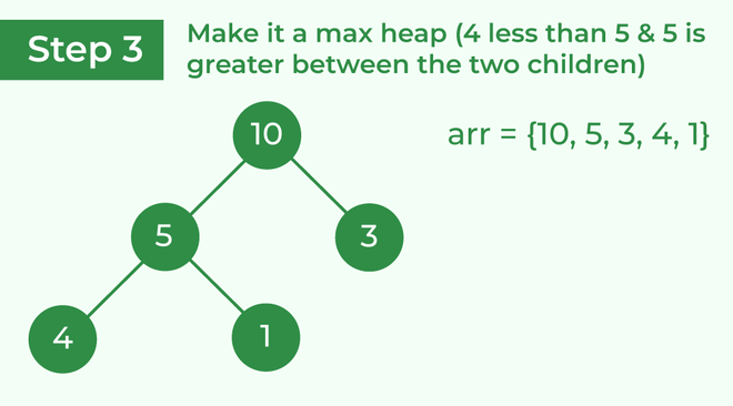
Make the tree a max heap

Perform heap sort: Remove the maximum element in each step (i.e., move it to the end position and remove that) and then consider the remaining elements and transform it into a max heap.

Delete the root element (10) from the max heap. In order to delete this node, try to swap it with the last node, i.e. (1). After removing the root element, again heapify it to convert it into max heap.
Resulted heap and array should look like this:
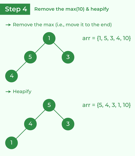
Remove 10 and perform heapify
Repeat the above steps and it will look like the following:
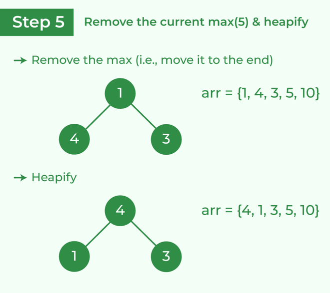
Remove 5 and perform heapify
Now remove the root (i.e. 3) again and perform heapify.
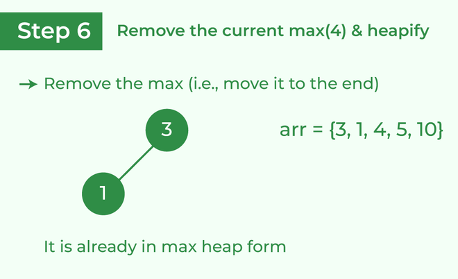
Remove 4 and perform heapify
Now when the root is removed once again it is sorted. and the sorted array will be like arr[] = {1, 3, 4, 5, 10}.
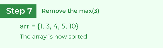
The sorted array

7. Counting sort

Counting sort is a sorting technique based on keys between a specific range. It works by counting the number of objects having distinct key values (kind of hashing). Then do some arithmetic to calculate the position of each object in the output sequence.

Working of Counting Sort algorithm:

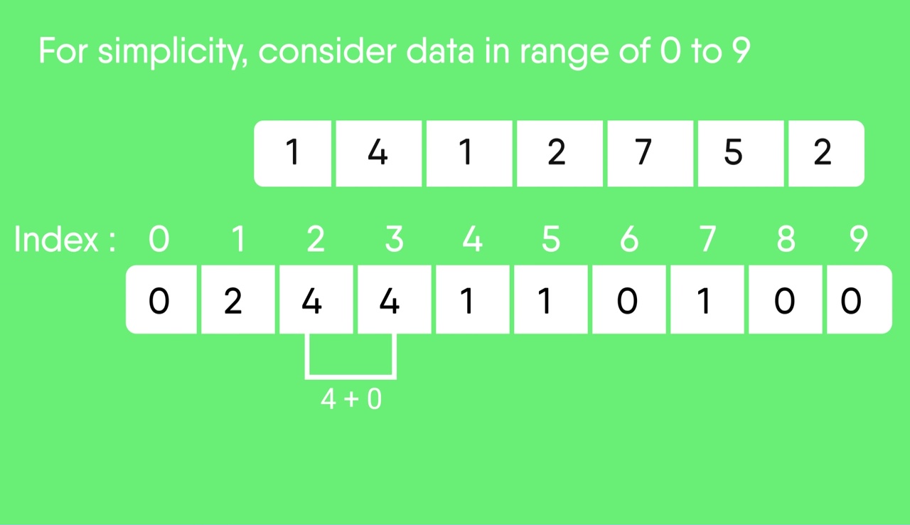
Consider the array: arr[] = {1, 4, 1, 2, 7, 5, 2}.

Input data: {1, 4, 1, 2, 7, 5, 2}
Take a count array to store the count of each unique object.

Now, store the count of each unique element in the count array
If any element repeats itself, simply increase its count.

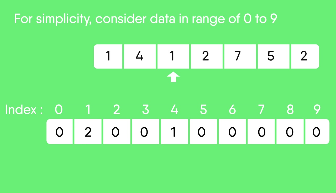
Here, the count of each unique element in the count array is as shown below:
Index: 0 1 2 3 4 5 6 7 8 9
Count: 0 2 2 0 1 1 0 1 0 0

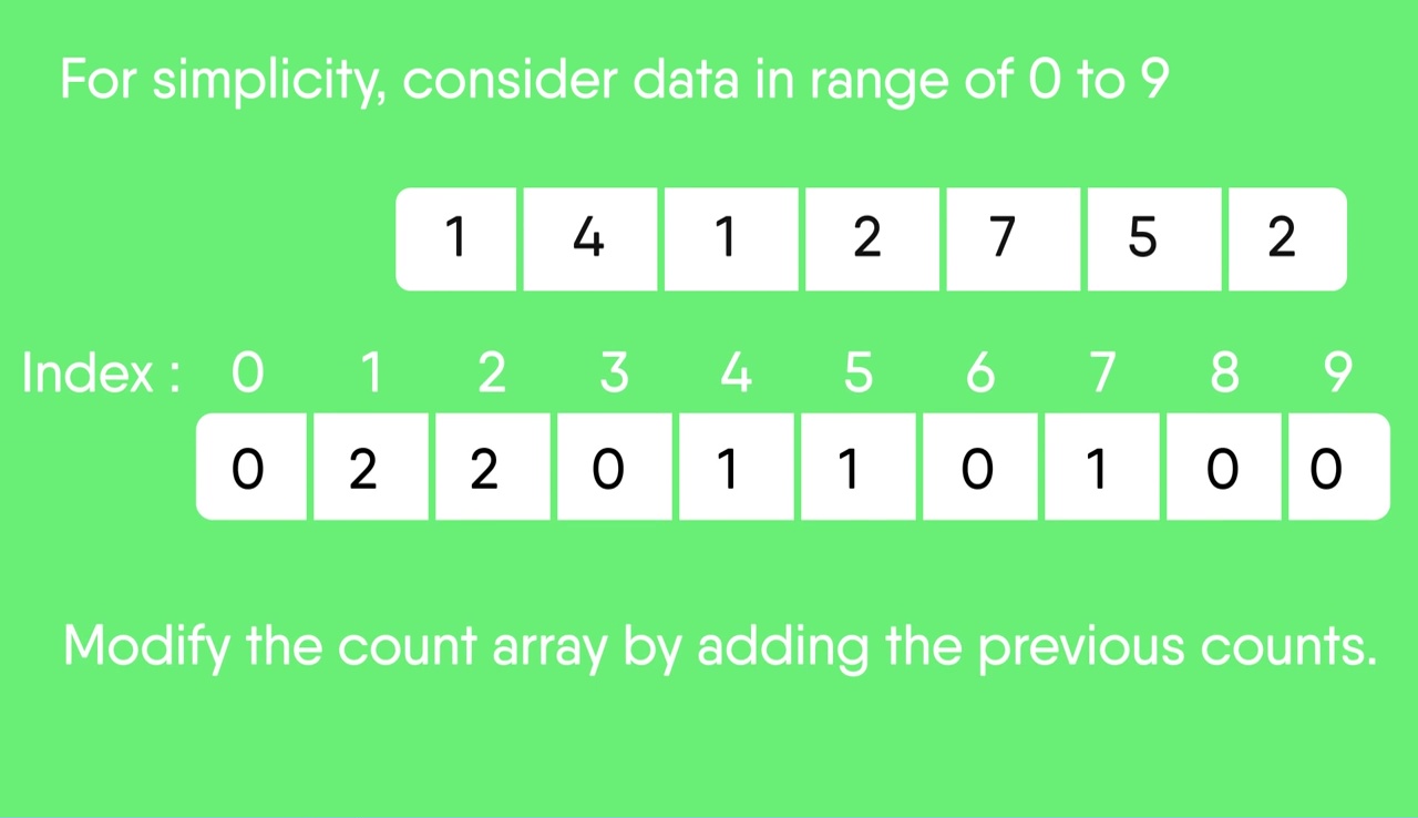
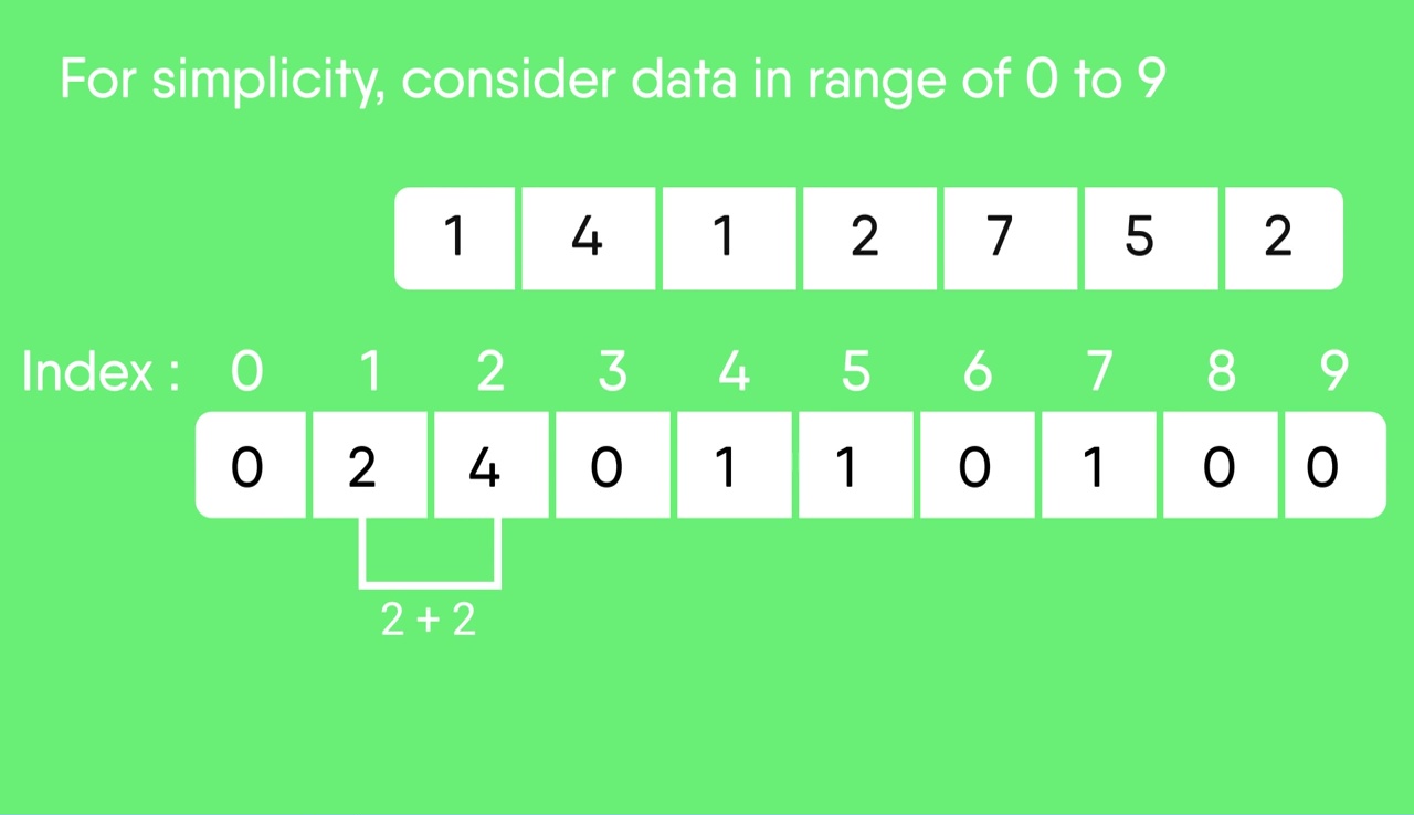
Modify the count array such that each element at each index stores the sum of previous counts.
Index: 0 1 2 3 4 5 6 7 8 9
Count: 0 2 4 4 5 6 6 7 7 7
The modified count array indicates the position of each object in the output sequence.
Find the index of each element of the original array in the count array. This gives the cumulative count.

Rotate the array clockwise for one time.
Index: 0 1 2 3 4 5 6 7 8 9
Count: 0 0 2 4 4 5 6 6 7 7

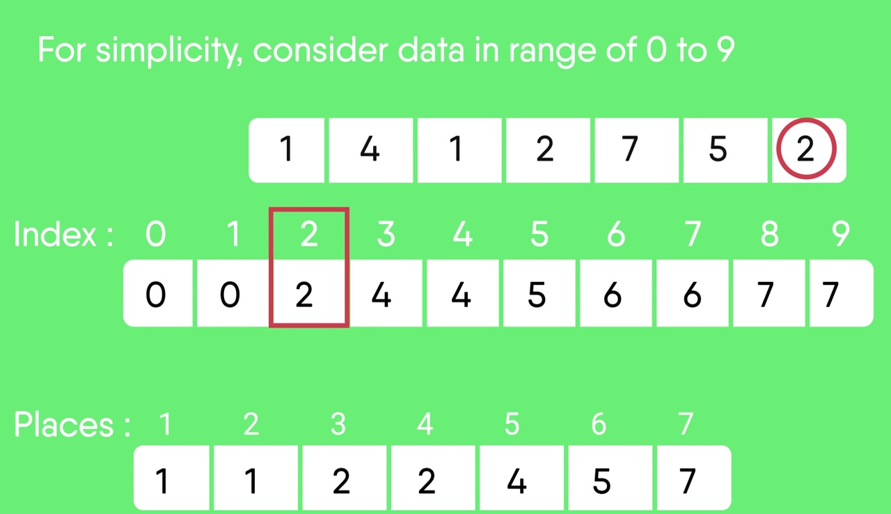
Output each object from the input sequence followed by increasing its count by 1.
Process the input data: 1, 4, 1, 2, 7, 5, 2. Position of 1 is 0.
Put data 1 at index 0 in output. Increase count by 1 to place next data 1 at an index 1 greater than this index.

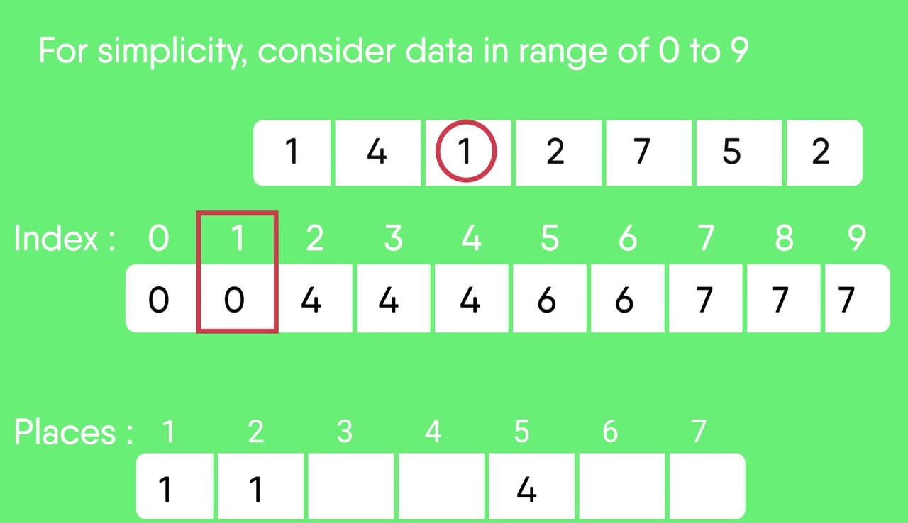
After placing each element at its correct position, decrease its count by one.

Some other Sorting algorithms:

1. Radix sort

Radix sort is a non-comparative sorting algorithm that is used to sort the data in lexicographical (dictionary) order.

It uses counting sort as a subroutine, to sort an array of integer digit by digit and array of strings character by character.

2. Bucket sort

Bucket Sort is a sorting algorithm that divides the unsorted array elements into several groups called buckets. Each bucket is then sorted by using any of the suitable sorting algorithms or recursively applying the same bucket algorithm.

Finally, the sorted buckets are combined to form a final sorted array.

3. Shell sort

Shell sort is mainly a variation of Insertion Sort. In insertion sort, we move elements only one position ahead. When an element has to be moved far ahead, many movements are involved. The idea of ShellSort is to allow the exchange of far items. In Shell sort, we make the array h-sorted for a large value of h. We keep reducing the value of h until it becomes 1. An array is said to be h-sorted if all sublists of every h’th element are sorted.

4. Tim Sort

Timsort is a hybrid sorting algorithm. It is used to give optimal results while dealing with real-world data.

Timsort has been derived from Insertion Sort and Binary Merge Sort. At first, the array is stored into smaller chunks of data known as runs. These runs are sorted using insertion sort and then merged using the merge sort.

5. Comb Sort

Comb Sort is mainly an improvement over Bubble Sort. Bubble sort always compares adjacent values. So all inversions are removed one by one. Comb Sort improves on Bubble Sort by using a gap of the size of more than 1. The gap starts with a large value and shrinks by a factor of 1.3 in every iteration until it reaches the value 1. Thus Comb Sort removes more than one inversion count with one swap and performs better than Bubble Sort.

6. Pigeonhole sorting

Pigeonhole sorting is a sorting algorithm that is suitable for sorting lists of elements where the number of elements and the number of possible key values are approximately the same.

7. Cycle Sort

Cycle sort is an in-place sorting Algorithm, unstable sorting algorithm, and a comparison sort that is theoretically optimal in terms of the total number of writes to the original array.

8. Cocktail Sort

Cocktail Sort is a variation of Bubble sort. The Bubble sort algorithm always traverses elements from left and moves the largest element to its correct position in the first iteration and second-largest in the second iteration and so on. Cocktail Sort traverses through a given array in both directions alternatively. Cocktail sort does not go through the unnecessary iteration making it efficient for large arrays.

Cocktail sorts break down barriers that limit bubble sorts from being efficient enough on large arrays by not allowing them to go through unnecessary iterations on one specific region (or cluster) before moving onto another section of an array.

9. Strand sort

Strand sort is a recursive sorting algorithm that sorts items of a list into increasing order. It has O(n²) worst time complexity which occurs when the input list is reverse sorted. It has a best case time complexity of O(n) which occurs when the input is a list that is already sorted.

10. Bitonic Sort

Bitonic Sort is a classic parallel algorithm for sorting.

The number of comparisons done by Bitonic sort is more than popular sorting algorithms like Merge Sort [ does O(log N) comparisons], but Bitonic sort is better for parallel implementation because we always compare elements in a predefined sequence and the sequence of comparison doesn’t depend on data. Therefore it is suitable for implementation in hardware and parallel processor array.
Bitonic Sort must be done if the number of elements to sort is 2^n. The procedure of bitonic sequence fails if the number of elements is not in the aforementioned quantity precisely.

11. Stooge Sort

Stooge Sort is a recursive sorting algorithm. It is not much efficient but an interesting sorting algorithm. It generally divides the array into two overlapping parts (2/3 each). After that it performs sorting in first 2/3 part and then it performs sorting in last 2/3 part. And then, sorting is done on first 2/3 part to ensure that the array is sorted.

The key idea is that sorting the overlapping part twice exchanges the elements between the other two sections accordingly.

12. Tag Sort

This is not a new sorting algorithm, but an idea when we need to avoid swapping of large objects or need to access elements of a large array in both original and sorted orders.
A common sorting task is to sort elements of an array using a sorting algorithm like Quick Sort, Bubble Sort.. etc, but there may be times when we need to keep the actual array intact and use a “tagged” array to store the correct positioning of the array when it is sorted. When we want to access elements in a sorted way, we can use this “tagged” array.

13. Tree sort

Tree sort is a sorting algorithm that is based on Binary Search Tree data structure. It first creates a binary search tree from the elements of the input list or array and then performs an in-order traversal on the created binary search tree to get the elements in sorted order.

14. Cartesian Sort

Cartesian Sort is an Adaptive Sorting as it sorts the data faster if data is partially sorted. In fact, there are very few sorting algorithms that make use of this fact. For example consider the array {5, 10, 40, 30, 28}. The input data is partially sorted too as only one swap between “40” and “28” results in a completely sorted order.

15. Odd-Even Sort / Brick Sort

This is basically a variation of bubble-sort. This algorithm is divided into two phases- Odd and Even Phase. The algorithm runs until the array elements are sorted and in each iteration two phases occurs- Odd and Even Phases.
In the odd phase, we perform a bubble sort on odd indexed elements and in the even phase, we perform a bubble sort on even indexed elements.

16. 3-way Merge Sort

Merge sort involves recursively splitting the array into 2 parts, sorting, and finally merging them. A variant of merge sort is called 3-way merge sort where instead of splitting the array into 2 parts we split it into 3 parts. Merge sort recursively breaks down the arrays to subarrays of size half. Similarly, the 3-way Merge sort breaks down the arrays to subarrays of size one-third.

17. Gnome sort

Gnome Sort also called Stupid sort is based on the concept of a Garden Gnome sorting his flower pots. A garden gnome sorts the flower pots by the following method-

He looks at the flower pot next to him and the previous one; if they are in the right order he steps one pot forward, otherwise, he swaps them and steps one pot backward.
If there is no previous pot (he is at the starting of the pot line), he steps forwards; if there is no pot next to him (he is at the end of the pot line), he is done.

18. Cocktail shaker sort

Cocktail Sort is a variation of Bubble sort. The Bubble sort algorithm always traverses elements from the left and moves the largest element to its correct position in the first iteration and the second-largest in the second iteration and so on. Cocktail Sort traverses through a given array in both directions alternatively. Cocktail sort does not go through the unnecessary iteration making it efficient for large arrays.

Comparison of Complexity Analysis Between Sorting Algorithms:

Name	Best Case	Average Case	Worst Case	Memory	Stable	Method Used
Quick Sort	$n log n$	$n log n$	$n^{2}$	$log n$	No	Partitioning
Merge Sort	$n log n$	$n log n$	$n log n$	n	Yes	Merging
Heap Sort	$n log n$	$n log n$	$n log n$	1	No	Selection
Insertion Sort	n	$n^{2}$	$n^{2}$	1	Yes	Insertion
Tim Sort	n	$n log n$	$n log n$	n	Yes	Insertion & Merging
Selection Sort	$n^{2}$	$n^{2}$	$n^{2}$	1	No	Selection
Shell Sort	$n log n$	$n^{4/3}$	$n^{3/2}$	1	No	Insertion
Bubble Sort	n	$n^{2}$	$n^{2}$	1	Yes	Exchanging
Tree Sort	$n log n$	$n log n$	$n log n$	n	Yes	Insertion
Cycle Sort	$n^{2}$	$n^{2}$	$n^{2}$	1	No	Selection
Strand Sort	n	$n^{2}$	$n^{2}$	n	Yes	Selection
Cocktail Shaker Sort	n	$n^{2}$	$n^{2}$	1	Yes	Exchanging
Comb Sort	$n log n$	$n^{2}$	$n^{2}$	1	No	Exchanging
Gnome Sort	n	$n^{2}$	$n^{2}$	1	Yes	Exchanging
Odd–even Sort	n	$n^{2}$	$n^{2}$	1	Yes	Exchanging

Suggest improvement

Sorting Algorithms

Selection Sort – Data Structure and Algorithm Tutorials

Share your thoughts in the comments

Most Common Sorting Algorithms

Other Sorting Algorithms

Comparison with other Sorting Algorithm

Easy problems on Sorting algorihtms

Medium problems on Sorting algorithms

Hard problem on Sorting algorithms