Branch and bound algorithms are used to find the optimal solution for combinatory, discrete, and general mathematical optimization problems.
A branch and bound algorithm provide an optimal solution to an NP-Hard problem by exploring the entire search space. Through the exploration of the entire search space, a branch and bound algorithm identify possible candidates for solutions step-by-step.
There are many optimization problems in computer science, many of which have a finite number of the feasible shortest path in a graph or minimum spanning tree that can be solved in polynomial time. Typically, these problems require a worst-case scenario of all possible permutations. The branch and bound algorithm create branches and bounds for the best solution.
In this tutorial, we’ll discuss the branch and bound method in detail.
Different search techniques in branch and bound:
The Branch algorithms incorporate different search techniques to traverse a state space tree. Different search techniques used in B&B are listed below:
- LC search
- BFS
- DFS
1. LC search (Least Cost Search):
It uses a heuristic cost function to compute the bound values at each node. Nodes are added to the list of live nodes as soon as they get generated.
The node with the least value of a cost function selected as a next E-node.
2.BFS(Breadth First Search):
It is also known as a FIFO search.
It maintains the list of live nodes in first-in-first-out order i.e, in a queue, The live nodes are searched in the FIFO order to make them next E-nodes.
3. DFS (Depth First Search):
It is also known as a LIFO search.
It maintains the list of live nodes in last-in-first-out order i.e. in a stack.
The live nodes are searched in the LIFO order to make them next E-nodes.

Introduction to Branch and Bound
When to apply Branch and Bound Algorithm?
Branch and bound is an effective solution to some problems, which we have already discussed. We’ll discuss all such cases where branching and binding are appropriate in this section.
- It is appropriate to use a branch and bound approach if the given problem is discrete optimization. Discrete optimization refers to problems in which the variables belong to the discrete set. Examples of such problems include 0-1 Integer Programming and Network Flow problems.
- When it comes to combinatory optimization problems, branch and bound work well. An optimization problem is optimized by combinatory optimization by finding its maximum or minimum based on its objective function. The combinatory optimization problems include Boolean Satisfiability and Integer Linear Programming.
Basic Concepts of Branch and Bound:
▸ Generation of a state space tree:
As in the case of backtracking, B&B generates a state space tree to efficiently search the solution space of a given problem instance.
In B&B, all children of an E-node in a state space tree are produced before any live node gets converted in an E-node. Thus, the E-node remains an E-node until i becomes a dead node.
- Evaluation of a candidate solution:
Unlike backtracking, B&B needs additional factors evaluate a candidate solution:
- A way to assign a bound on the best values of the given criterion functions to each node in a state space tree: It is produced by the addition of further components to the partial solution given by that node.
- The best values of a given criterion function obtained so far: It describes the upper bound for the maximization problem and the lower bound for the minimization problem.
- A feasible solution is defined by the problem states that satisfy all the given constraints.
- An optimal solution is a feasible solution, which produces the best value of a given objective function.
- Bounding function :
It optimizes the search for a solution vector in the solution space of a given problem instance.
It is a heuristic function that evaluates the lower and upper bounds on the possible solutions at each node. The bound values are used to search the partial solutions leading to an optimal solution. If a node does not produce a solution better than the best solution obtained thus far, then it is abandoned without further exploration.
The algorithm then branches to another path to get a better solution. The desired solution to the problem is the value of the best solution produced so far.
▸ The reasons to dismiss a search path at the current node :
(i) The bound value of the node is lower than the upper bound in the case of the maximization problem and higher than the lower bound in the case of the minimization problem. (i.e. the bound value of the ade is not better than the value of the best solution obtained until that node).
(ii) The node represents infeasible solutions, de violation of the constraints of the problem.
(iii) The node represents a subset of a feasible solution containing a single point. In this case, if the latest solution is better than the best solution obtained so far the best solution is modified to the value of a feasible solution at that node.
Types of Branch and Bound Solutions:
The solution of the Branch and the bound problem can be represented in two ways:
- Variable size solution: Using this solution, we can find the subset of the given set that gives the optimized solution to the given problem. For example, if we have to select a combination of elements from {A, B, C, D} that optimizes the given problem, and it is found that A and B together give the best solution, then the solution will be {A, B}.
- Fixed-size solution: There are 0s and 1s in this solution, with the digit at the ith position indicating whether the ith element should be included, for the above example, the solution will be given by {1, 1, 0, 0}, here 1 represent that we have select the element which at ith position and 0 represent we don’t select the element at ith position.
Classification of Branch and Bound Problems:
The Branch and Bound method can be classified into three types based on the order in which the state space tree is searched.
- FIFO Branch and Bound
- LIFO Branch and Bound
- Least Cost-Branch and Bound
We will now discuss each of these methods in more detail. To denote the solutions in these methods, we will use the variable solution method.
1. FIFO Branch and Bound
First-In-First-Out is an approach to the branch and bound problem that uses the queue approach to create a state-space tree. In this case, the breadth-first search is performed, that is, the elements at a certain level are all searched, and then the elements at the next level are searched, starting with the first child of the first node at the previous level.
For a given set {A, B, C, D}, the state space tree will be constructed as follows :
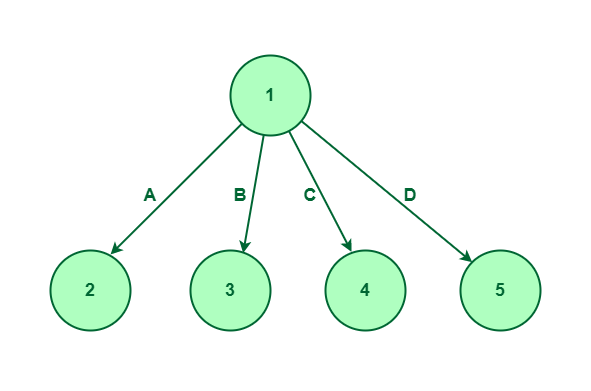
State Space tree for set {A, B, C, D}
The above diagram shows that we first consider element A, then element B, then element C and finally we’ll consider the last element which is D. We are performing BFS while exploring the nodes.
So, once the first level is completed. We’ll consider the first element, then we can consider either B, C, or D. If we follow the route then it says that we are doing elements A and D so we will not consider elements B and C. If we select the elements A and D only, then it says that we are selecting elements A and D and we are not considering elements B and C.
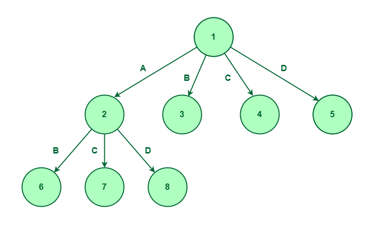
Selecting element A
Now, we will expand node 3, as we have considered element B and not considered element A, so, we have two options to explore that is elements C and D. Let’s create nodes 9 and 10 for elements C and D respectively.
Considered element B and not considered element A
Now, we will expand node 4 as we have only considered elements C and not considered elements A and B, so, we have only one option to explore which is element D. Let’s create node 11 for D.
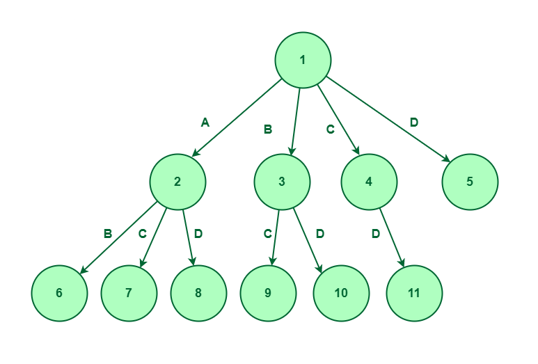
Considered elements C and not considered elements A and B
Till node 5, we have only considered elements D, and not selected elements A, B, and C. So, We have no more elements to explore, Therefore on node 5, there won’t be any expansion.
Now, we will expand node 6 as we have considered elements A and B, so, we have only two option to explore that is element C and D. Let’s create node 12 and 13 for C and D respectively.
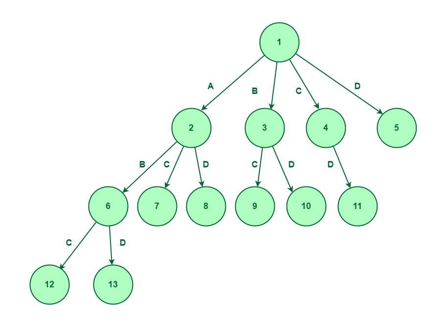
Expand node 6
Now, we will expand node 7 as we have considered elements A and C and not consider element B, so, we have only one option to explore which is element D. Let’s create node 14 for D.
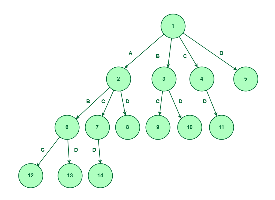
Expand node 7
Till node 8, we have considered elements A and D, and not selected elements B and C, So, We have no more elements to explore, Therefore on node 8, there won’t be any expansion.
Now, we will expand node 9 as we have considered elements B and C and not considered element A, so, we have only one option to explore which is element D. Let’s create node 15 for D.
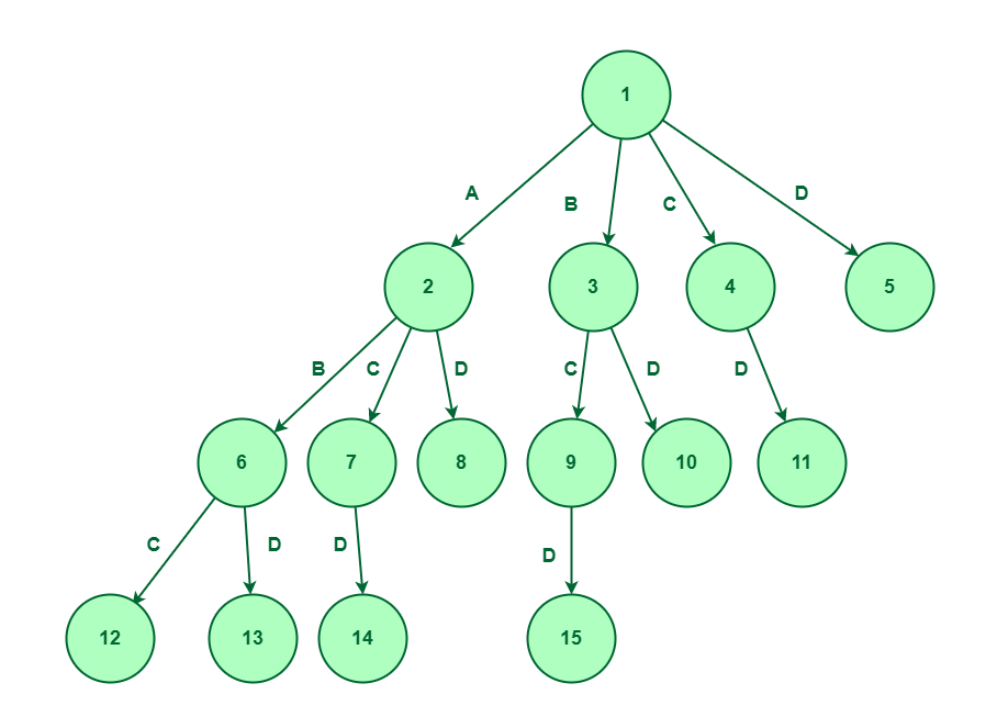
Expand node 9
2. LIFO Branch and Bound
The Last-In-First-Out approach for this problem uses stack in creating the state space tree. When nodes are added to a state space tree, they are added to a stack. After all nodes of a level have been added, we pop the topmost element from the stack and explore it.
For a given set {A, B, C, D}, the state space tree will be constructed as follows :
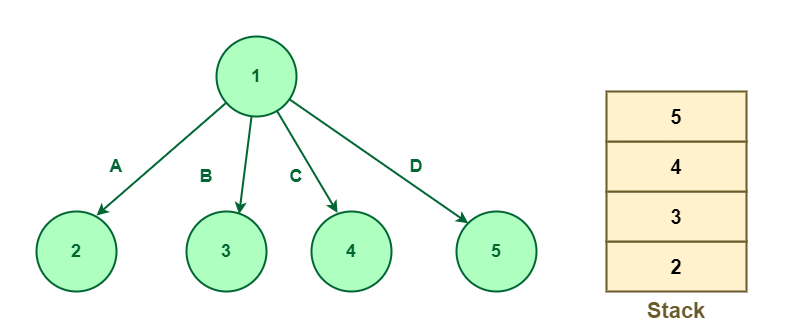
State space tree for element {A, B, C, D}
Now the expansion would be based on the node that appears on the top of the stack. Since node 5 appears on the top of the stack, so we will expand node 5. We will pop out node 5 from the stack. Since node 5 is in the last element, i.e., D so there is no further scope for expansion.
The next node that appears on the top of the stack is node 4. Pop-out node 4 and expand. On expansion, element D will be considered and node 6 will be added to the stack shown below:
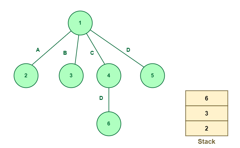
Expand node 4
The next node is 6 which is to be expanded. Pop-out node 6 and expand. Since node 6 is in the last element, i.e., D so there is no further scope for expansion.
The next node to be expanded is node 3. Since node 3 works on element B so node 3 will be expanded to two nodes, i.e., 7 and 8 working on elements C and D respectively. Nodes 7 and 8 will be pushed into the stack.
The next node that appears on the top of the stack is node 8. Pop-out node 8 and expand. Since node 8 works on element D so there is no further scope for the expansion.
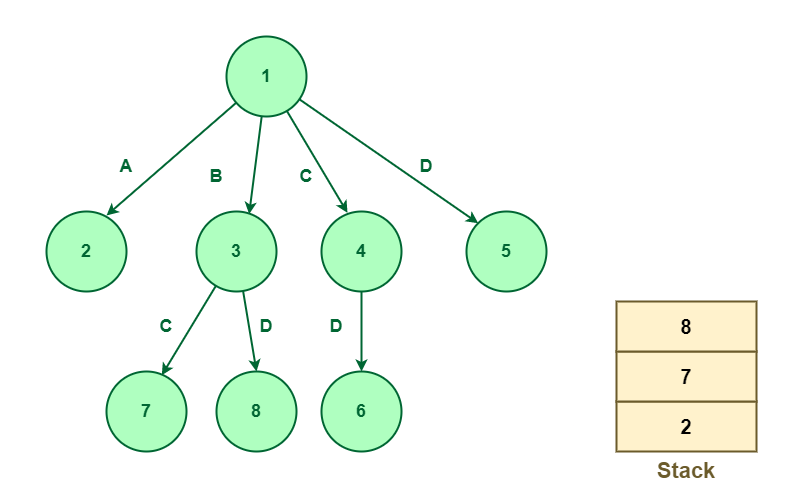
Expand node 3
The next node that appears on the top of the stack is node 7. Pop-out node 7 and expand. Since node 7 works on element C so node 7 will be further expanded to node 9 which works on element D and node 9 will be pushed into the stack.
The next node is 6 which is to be expanded. Pop-out node 6 and expand. Since node 6 is in the last element, i.e., D so there is no further scope for expansion.
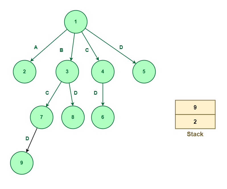
Expand node 7
The next node that appears on the top of the stack is node 9. Since node 9 works on element D, there is no further scope for expansion.
The next node that appears on the top of the stack is node 2. Since node 2 works on the element A so it means that node 2 can be further expanded. It can be expanded up to three nodes named 10, 11, 12 working on elements B, C, and D respectively. There new nodes will be pushed into the stack shown as below:
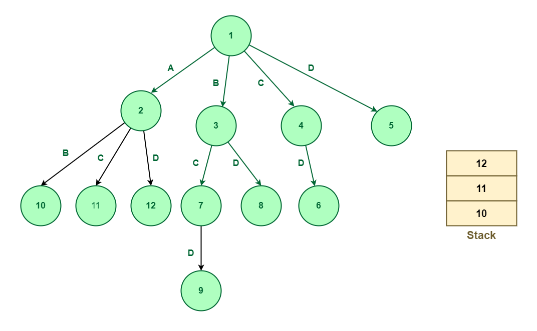
Expand node 2
In the above method, we explored all the nodes using the stack that follows the LIFO principle.
3. Least Cost-Branch and Bound
To explore the state space tree, this method uses the cost function. The previous two methods also calculate the cost function at each node but the cost is not been used for further exploration.
In this technique, nodes are explored based on their costs, the cost of the node can be defined using the problem and with the help of the given problem, we can define the cost function. Once the cost function is defined, we can define the cost of the node.
Now, Consider a node whose cost has been determined. If this value is greater than U0, this node or its children will not be able to give a solution. As a result, we can kill this node and not explore its further branches. As a result, this method prevents us from exploring cases that are not worth it, which makes it more efficient for us.
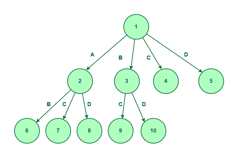
Let’s first consider node 1 having cost infinity shown below:
In the following diagram, node 1 is expanded into four nodes named 2, 3, 4, and 5.
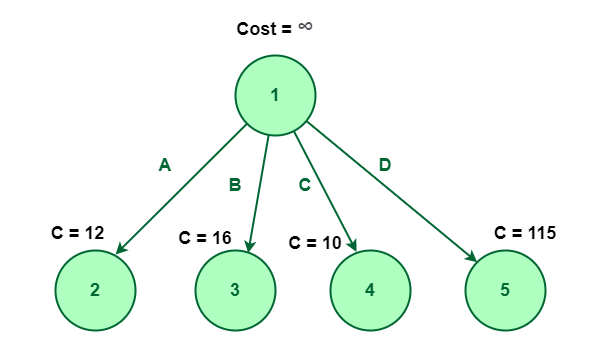
Node 1 is expanded into four nodes named 2, 3, 4, and 5
Assume that cost of the nodes 2, 3, 4, and 5 are 12, 16, 10, and 315 respectively.
In this method, we will explore the node which is having the least cost. In the above figure, we can observe that the node with a minimum cost is node 4. So, we will explore node 4 having a cost of 10.
During exploring node 4 which is element C, we can notice that there is only one possible element that remains unexplored which is D (i.e, we already decided not to select elements A, and B). So, it will get expanded to one single element D, let’s say this node number is 6.
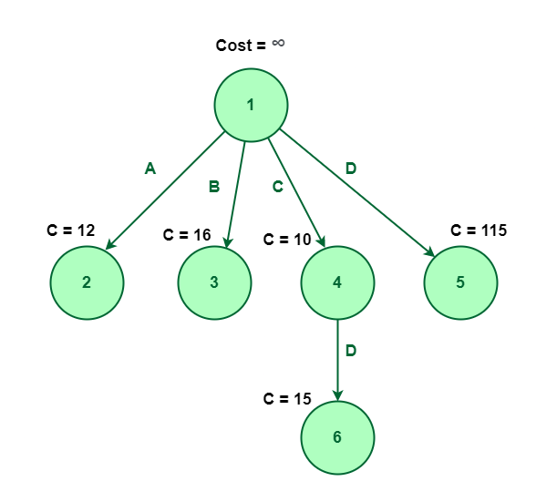
Exploring node 4 which is element C
Now, Node 6 has no element left to explore. So, there is no further scope for expansion. Hence the element {C, D} is the optimal way to choose for the least cost.
Problems that can be solved using Branch and Bound Algorithm:
The Branch and Bound method can be used for solving most combinatorial problems. Some of these problems are given below:
Advantages of Branch and Bound Algorithm:
- We don’t explore all the nodes in a branch and bound algorithm. Due to this, the branch and the bound algorithm have a lower time complexity than other algorithms.
- Whenever the problem is small and the branching can be completed in a reasonable amount of time, the algorithm finds an optimal solution.
- By using the branch and bound algorithm, the optimal solution is reached in a minimal amount of time. When exploring a tree, it does not repeat nodes.
Disadvantages of Branch and Bound Algorithm:
- It takes a long time to run the branch and bound algorithm.
- In the worst-case scenario, the number of nodes in the tree may be too large based on the size of the problem.
Conclusion
The branch and bound algorithms are one of the most popular algorithms used in optimization problems that we have discussed in our tutorial. We have also explained when a branch and bound algorithm is appropriate for a user to use. In addition, we presented an algorithm based on branches and bounds for assigning jobs. Lastly, we discussed some advantages and disadvantages of branch and bound algorithms.
Like Article
Suggest improvement
Share your thoughts in the comments
Please Login to comment...