Interpreting the results of Linear Regression using OLS Summary

This article is to tell you the whole interpretation of the regression summary table. There are many statistical softwares that are used for regression analysis like Matlab, Minitab, spss, R etc. but this article uses python. The Interpretation is the same for other tools as well. This article needs the basics of statistics including basic knowledge of regression, degrees of freedom, standard deviation, Residual Sum Of Squares(RSS), ESS, t statistics etc. 

In regression there are two types of variables i.e. dependent variable (also called explained variable) and independent variable (explanatory variable). 

The regression line used here is,

The summary table of the regression is given below.

                                    OLS Regression Results                            
        ==============================================================================
        Dep. Variable:                      y   R-squared:                       0.669
        Model:                            OLS   Adj. R-squared:                  0.667
        Method:                 Least Squares   F-statistic:                     299.2
        Date:                Mon, 01 Mar 2021   Prob (F-statistic):           2.33e-37
        Time:                        16:19:34   Log-Likelihood:                -88.686
        No. Observations:                 150   AIC:                             181.4
        Df Residuals:                     148   BIC:                             187.4
        Df Model:                           1                                         
        Covariance Type:            nonrobust                                         
        ==============================================================================
                         coef    std err          t      P>|t|      [0.025      0.975]
        ------------------------------------------------------------------------------
        const         -3.2002      0.257    -12.458      0.000      -3.708      -2.693
        x1             0.7529      0.044     17.296      0.000       0.667       0.839
        ==============================================================================
        Omnibus:                        3.538   Durbin-Watson:                   1.279
        Prob(Omnibus):                  0.171   Jarque-Bera (JB):                3.589
        Skew:                           0.357   Prob(JB):                        0.166
        Kurtosis:                       2.744   Cond. No.                         43.4
        ==============================================================================

Dependent variable: Dependent variable is one that is going to depend on other variables. In this regression analysis Y is our dependent variable because we want to analyse the effect of X on Y.

Model: The method of Ordinary Least Squares(OLS) is most widely used model due to its efficiency. This model gives best approximate of true population regression line. The principle of OLS is to minimize the square of errors ( ∑e_i² ).

Number of observations: The number of observation is the size of our sample, i.e. N = 150.

Degree of freedom(df) of residuals: 

Degree of freedom is the number of independent observations on the basis of which the sum of squares is calculated.

D.f Residuals = 150 – (1+1) = 148

Degree of freedom(D.f) is calculated as,      

 Degrees of freedom,  D . f  = N – K

Where, N = sample size(no. of observations) and  K = number of variables + 1

Df of model: 

Df of model = K – 1 = 2 – 1 = 1 ,

Where, K = number of variables + 1

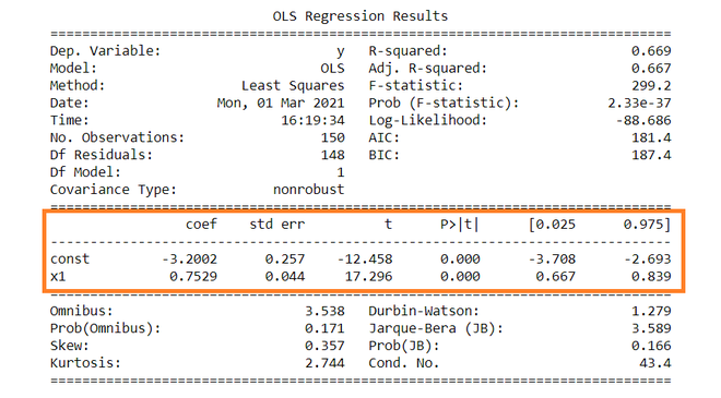
Constant term: The constant terms is the intercept of the regression line. From regression line (eq…1) the intercept is -3.002. In regression we omits some independent variables that do not have much impact on the dependent variable, the intercept tells the average value of these omitted variables and noise present in model.

Coefficient term: The coefficient term tells the change in Y for a unit change in X  i.e if X rises by 1 unit then Y rises by 0.7529. If you are familiar with derivatives then you can relate it as the rate of change of Y with respect to X .

Standard error of parameters: Standard error is also called the standard deviation. Standard error shows the sampling variability of these parameters. Standard error is calculated by as – 

Standard error of intercept term (b1): 

Standard error of coefficient term(b2): 

Here,  σ² is the Standard error of regression (SER) .  And σ² is equal to RSS( Residual Sum Of Square i.e ∑e_i² ).

t – statistics: 

In theory, we assume that error term follows the normal distribution and because of this the parameters b₁  and  b₂ also have normal distributions with variance calculated in above section.

 That is , 

• b₁  ∼ N(B₁, σ_b1²)
• b₂   ∼ N(B_{2 ,} σ_b2²)

Here B₁ and B₂  are true means of b1 and  b2.

t – statistics are calculated by assuming  following hypothesis – 

• H₀  : B₂  = 0       ( variable X has no influence on Y)
• H_a  : B₂  ≠ 0      (X has significant impact on Y)

Calculations for t – statistics :          

t = ( b₁ – B₁ ) / s.e (b₁)

From summary table , b₁ = -3.2002 and se(b₁) = 0.257, So,

t = (-3.2002 – 0) / 0.257  = -12.458

Similarly,  b₂ = 0.7529 , se(b₂) = 0.044

                   t = (0.7529 – 0) / 0.044  = 17.296

p – values: 

In theory, we read that p-value is the probability of obtaining the t statistics at least as contradictory to H₀  as calculated from assuming that the null hypothesis is true. In the summary table, we can see that P-value for both parameters is equal to 0. This is not exactly 0, but since we have very larger statistics (-12.458 and 17.296) p-value will be approximately 0.

If you know about significance levels then you can see that we can reject the null hypothesis at almost every significance level.

Confidence intervals:

There are many approaches to test the hypothesis, including the p-value approach mentioned above. The confidence interval approach is one of them. 5% is the standard significance level (∝) at which C.I’s are made. 

C.I for B₁ is ( b₁ – t_∝/2 s.e(b₁) , b₁ + t_∝/2 s.e(b₁) )

Since ∝ = 5 %, b₁ = -3.2002, s.e(b₁) =0.257 , from t table , t_0.025,148 = 1.655,

After putting values the C.I for B₁ is approx. ( -3.708 , -2.693 ). Same can be done for b₂ as well.

While calculating p values we rejected the null hypothesis we can see same in C.I as well. Since 0 does not lie in any of the intervals so we will reject the null hypothesis. 

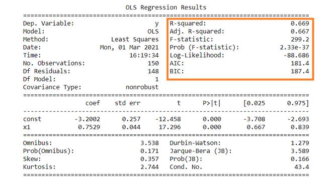
 R – squared value: 

R² is the coefficient of determination that tells us that how much percentage variation independent variable can be explained by independent variable. Here, 66.9 % variation in Y can be explained by X. The maximum possible value of R²  can be 1, means the larger the R²  value better the regression.

F – statistic: 

F test tells the goodness of fit of a regression. The test is similar to the t-test or other tests we do for the hypothesis. The F – statistic is calculated as below –                    

Inserting the values of R², n and k, F = (0.669/1) / (0.331/148) = 229.12.

You can calculate the probability of F >229.1 for 1 and 148 df, which comes to approx. 0. From this, we again reject the null hypothesis stated above. 

The remaining terms are not often used. Terms like Skewness and Kurtosis tells about the distribution of data. Skewness and kurtosis for the normal distribution are 0 and 3 respectively. Jarque-Bera test is used for checking whether an error has normal distribution or not.