Inception V2 and V3 – Inception Network Versions
Last Updated :
14 Oct, 2022
Inception V1 (or GoogLeNet) was the state-of-the-art architecture at ILSRVRC 2014. It has produced the record lowest error at ImageNet classification dataset but there are some points on which improvement can be made to improve the accuracy and decrease the complexity of the model.
Problems of Inception V1 architecture:
Inception V1 have sometimes use convolutions such as 5*5 that causes the input dimensions to decrease by a large margin. This causes the neural network to uses some accuracy decrease. The reason behind that the neural network is susceptible to information loss if the input dimension decreases too drastically.
Furthermore, there is also a complexity decrease when we use bigger convolutions like 5×5 as compared to 3×3. We can go further in terms of factorization i.e. that we can divide a 3×3 convolution into an asymmetric convolution of 1×3 then followed by a 3×1 convolution. This is equivalent to sliding a two-layer network with the same receptive field as in a 3×3 convolution but 33% cheaper than 3×3. This factorization does not work well for early layers when input dimensions are big but only when the input size mxm (m is between 12 and 20). According to the Inception V1 architecture, the auxiliary classifier improves the convergence of the network. They argue that it can help reduce the effect of the vanishing gradient problem in the deep networks by pushing the useful gradient to earlier layers (to reduce the loss). But, the authors of this paper found that this classifier didn’t improve the convergence very much early in the training.
Architectural Changes in Inception V2:
In the Inception V2 architecture. The 5×5 convolution is replaced by the two 3×3 convolutions. This also decreases computational time and thus increases computational speed because a 5×5 convolution is 2.78 more expensive than a 3×3 convolution. So, Using two 3×3 layers instead of 5×5 increases the performance of architecture.
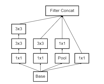
Figure 1
This architecture also converts nXn factorization into 1xn and nx1 factorization. As we discussed above that a 3×3 convolution can be converted into 1×3 then followed by 3×1 convolution which is 33% cheaper in terms of computational complexity as compared to 3×3.
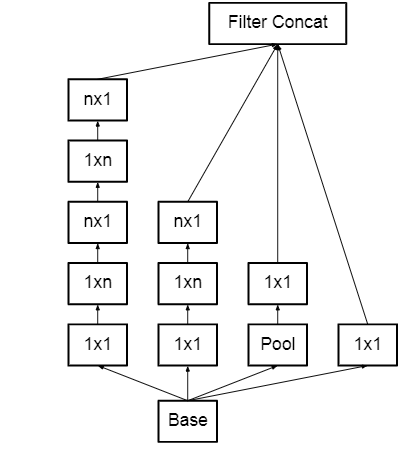
Figure 2
To deal with the problem of the representational bottleneck, the feature banks of the module were expanded instead of making it deeper. This would prevent the loss of information that causes when we make it deeper.
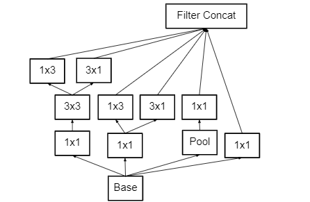
Figure 3
Architectural Changes in Inception V3:
Inception V3 is similar to and contains all the features of Inception V2 with following changes/additions:
- Use of RMSprop optimizer.
- Batch Normalization in the fully connected layer of Auxiliary classifier.
- Use of 7×7 factorized Convolution
- Label Smoothing Regularization: It is a method to regularize the classifier by estimating the effect of label-dropout during training. It prevents the classifier to predict a class too confidently. The addition of label smoothing gives 0.2% improvement from the error rate.
Architecture:
Below is the layer-by-layer details of Inception V2:
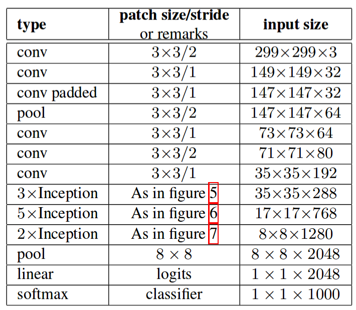
Inception V2 architecture
The above architecture takes image input of size (299,299,3). Notice in the above architecture figures 5, 6, 7 refers to figure 1, 2, 3 in this article.
Implementation:
In this section we will look into the implementation of Inception V3. We will using Keras applications API to load the module We are using Cats vs Dogs dataset for this implementation.
Code: Importing the required module.
python3
import os
import zipfile
import tensorflow as tf
from tensorflow.keras.optimizers import RMSprop
from tensorflow.keras.preprocessing.image import ImageDataGenerator
from tensorflow.keras import layers
from tensorflow.keras import Model
from tensorflow.keras.applications.inception_v3 import InceptionV3
from tensorflow.keras.optimizers import RMSprop
|
Code: Creating directories in order to prepare for the dataset
python3
local_zip = '/dataset/cats_and_dogs_filtered.zip'
zip_ref = zipfile.ZipFile(local_zip, 'r')
zip_ref.extractall('/tmp')
zip_ref.close()
base_dataset_dir = '/tmp/cats_and_dogs_filtered'
train_dir = os.path.join(base_dataset_dir, 'train')
validation_dir = os.path.join(base_dataset_dir, 'validation')
train_cats = os.path.join(train_dir, 'cats')
train_dogs = os.path.join(train_dir, 'dogs')
validation_cats = os.path.join(validation_dir, 'cats')
validation_dogs = os.path.join(validation_dir, 'dogs')
|
Code: Storing the dataset in the directories created above and plot some sample images.
python3
import matplotlib.image as mpimg
nrows = 4
ncols = 4
fig = plt.gcf()
fig.set_size_inches(ncols*4, nrows*4)
pic_index = 100
train_cat_files = os.listdir( train_cats )
train_dog_files = os.listdir( train_dogs )
next_cat_img = [os.path.join(train_cats, fname)
for fname in train_cat_files[ pic_index-8:pic_index]
]
next_dog_img = [os.path.join(train_dogs, fname)
for fname in train_dog_files[ pic_index-8:pic_index]
]
for i, img_path in enumerate(next_cat_img+next_dog_img):
sp = plt.subplot(nrows, ncols, i + 1)
sp.axis('Off')
img = mpimg.imread(img_path)
plt.imshow(img)
plt.show()
|
Code: Data augmentation to increase the data samples in dataset.
python3
train_datagen = ImageDataGenerator(rescale = 1./255.,
rotation_range = 50,
width_shift_range = 0.2,
height_shift_range = 0.2,
zoom_range = 0.2,
horizontal_flip = True)
test_datagen = ImageDataGenerator( rescale = 1.0/255. )
train_generator = train_datagen.flow_from_directory(train_dir,
batch_size = 20,
class_mode = 'binary',
target_size = (150, 150))
validation_generator = test_datagen.flow_from_directory( validation_dir,
batch_size = 20,
class_mode = 'binary',
target_size = (150, 150))
|
Code: Define the base model using Inception API we imported above and callback function to train the model.
python3
base_model = InceptionV3(input_shape = (150, 150, 3),
include_top = False,
weights = 'imagenet')
for layer in base_model.layers:
layer.trainable = False
class myCallback(tf.keras.callbacks.Callback):
def on_epoch_end(self, epoch, logs={}):
if(logs.get('acc')>0.99):
self.model.stop_training = True
|
In this step, we train our model but before training, we need to change the last layer so that it can predict only one output and use the optimizer function for training. Here we used RMSprop with a learning rate of 0.0001. We also add a dropout 0.2 after the last fully connected layer. After that, we train the model up to 100 epochs.
Code:
python3
x = layers.Flatten()(base_model.output)
x = layers.Dense(1024, activation='relu')(x)
x = layers.Dropout(0.2)(x)
x = layers.Dense (1, activation='sigmoid')(x)
model = Model( base_model.input, x)
model.compile(optimizer = RMSprop(lr=0.0001),loss = 'binary_crossentropy',metrics = ['acc'])
callbacks = myCallback()
history = model.fit_generator(
train_generator,
validation_data = validation_generator,
steps_per_epoch = 100,
epochs = 100,
validation_steps = 50,
verbose = 2,
callbacks=[callbacks])
|
Code: Plot the training and validation accuracy along with training and validation loss.
python3
acc = history.history['acc']
val_acc = history.history['val_acc']
loss = history.history['loss']
val_loss = history.history['val_loss']
epochs = range(len(acc))
plt.plot(epochs, acc, 'r', label='Training accuracy')
plt.plot(epochs, val_acc, 'b', label='Validation accuracy')
plt.title('Training and validation accuracy')
plt.figure()
plt.plot(epochs, loss, 'r', label='Training Loss')
plt.plot(epochs, val_loss, 'b', label='Validation Loss')
plt.title('Training and validation loss')
plt.legend()
|
Results:
The best performing Inception V3 architecture reported top-5 error of just 5.6% and top-1 error of 21.2% for a single crop on ILSVRC 2012 classification challenge which is the new state-of-the-art. On multiple crops(144 crops) it reported top-5 and top-1 error rate of 4.2% and 18.77% on ILSVRC 2012 classification benchmark.

Inception V3 Performance
An ensemble of Inception V3 architecture reported a top-5 error rate of 3.46% ILSVRC 2012 validation set (3.58% on ILSVRC 2012 test set).
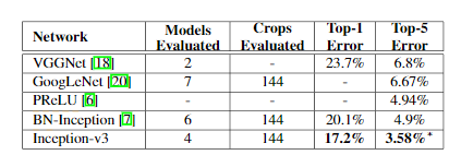
Ensemble Results of Inception V3
References:
Like Article
Suggest improvement
Share your thoughts in the comments
Please Login to comment...