Implementing Models of Artificial Neural Network

1. McCulloch-Pitts Model of Neuron

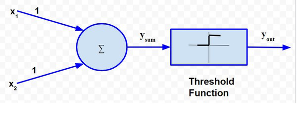
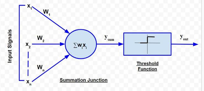
The McCulloch-Pitts neural model, which was the earliest ANN model, has only two types of inputs — Excitatory and Inhibitory. The excitatory inputs have weights of positive magnitude and the inhibitory weights have weights of negative magnitude. The inputs of the McCulloch-Pitts neuron could be either 0 or 1. It has a threshold function as an activation function. So, the output signal y_out is 1 if the input y_sum is greater than or equal to a given threshold value, else 0. The diagrammatic representation of the model is as follows:

McCulloch-Pitts Model

Simple McCulloch-Pitts neurons can be used to design logical operations. For that purpose, the connection weights need to be correctly decided along with the threshold function (rather than the threshold value of the activation function). For better understanding purpose, let me consider an example:

John carries an umbrella if it is sunny or if it is raining. There are four given situations. I need to decide when John will carry the umbrella. The situations are as follows:

• First scenario: It is not raining, nor it is sunny
• Second scenario: It is not raining, but it is sunny
• Third scenario: It is raining, and it is not sunny
• Fourth scenario: It is raining as well as it is sunny

To analyse the situations using the McCulloch-Pitts neural model, I can consider the  input signals as follows:

• X₁: Is it raining?
• X₂ : Is it sunny?

So, the value of both scenarios can be either 0 or 1. We can use the value of both weights X₁ and X₂ as 1 and a threshold function as 1. So, the neural network model will look like:

Truth Table for this case will be: 

Situation	x1	x2	ysum	yout
1	0	0	0	0
2	0	1	1	1
3	1	0	1	1
4	1	1	2	1

So, I can say that,

[Tex]y_{sum} = \sum_{i=1}^2w_ix_i [/Tex]

[Tex]y_{out}=f(y_{sum})=\bigg\{\begin{matrix} 1, x \geq 1 \\ 0, x < 1 \end{matrix} [/Tex]

The truth table built with respect to the problem is depicted above. From the truth table, I can conclude that in the situations where the value of y_out is 1, John needs to carry an umbrella. Hence, he will need to carry an umbrella in scenarios 2, 3 and 4. 

Python3

import tensorflow as tf def mcculloh_pits_neuron(inputs,weights,threshold): weighted_sum = tf.reduce_sum(tf.multiply(inputs,weights)) output = tf.cond(weighted_sum >= threshold,lambda:1.0,lambda:0.0) return output inputs = tf.constant([0.5,0.3,0.8],dtype=tf.float32) weights = tf.constant([0.2,0.4,0.6],dtype=tf.float32) threshold = tf.constant(0.7,dtype=tf.float32) output = mcculloh_pits_neuron(inputs,weights,threshold) print("output",output)

output: 1.0

2. Rosenblatt’s Perceptron

Rosenblatt’s perceptron is built around the McCulloch-Pitts neural model. The diagrammatic representation is as follows:

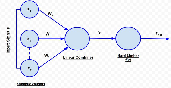
Rosenblatt’s Perceptron

The perceptron receives a set of input x₁, x₂,….., x_n. The linear combiner or the adder mode computes the linear combination of the inputs applied to the synapses with synaptic weights being w₁, w₂,……,w_n. Then, the hard limiter checks whether the resulting sum is positive or negative If the input of the hard limiter node is positive, the output is +1, and if the input is negative, the output is -1. Mathematically  the hard limiter input is:

[Tex]v = \sum_{i=1}^nw_ix_i [/Tex]

However, perceptron includes an adjustable value or bias as an additional weight w₀. This additional weight is attached to a dummy input x₀, which is assigned a value of 1. This consideration modifies the above equation to:

[Tex]v = \sum_{i=0}^nw_ix_i [/Tex]

The output is decided by the expression:

[Tex]y_{out}=f(v)=\bigg\{\begin{matrix} +1, v > 0 \\ -1, v < 0 \end{matrix} [/Tex]

The objective of the perceptron is o classify a set of inputs into two classes c₁ and c₂. This can be done using a very simple decision rule – assign the inputs to c₁ if the output of the perceptron i.e. y_out is +1 and c₂ if y_out is -1. So for an n-dimensional signal space i.e. a space for ‘n’ input signals, the simplest form of perceptron will have two decision regions, resembling two classes, separated by a hyperplane defined by:

[Tex]\sum_{i=0}^nw_ix_i = 0 [/Tex]

Therefore, the two input signals denoted by the variables x₁ and x₂, the decision boundary is a straight line of the form:

[Tex]w_0x_0+w_1x_1+w_2x_2=0      [/Tex]  or

[Tex]w_0+w_1x_1+w_2x_2=0 [\because x_0 =1] [/Tex]

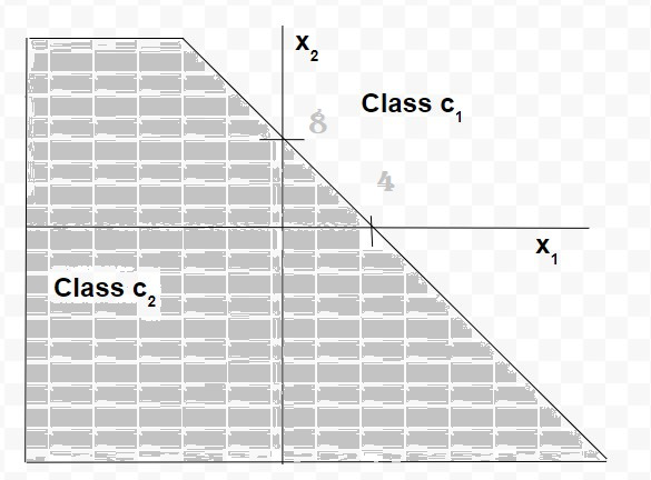
So, for a perceptron having the values of synaptic weights w₀,w₁ and w₂ as -2, 1/2 and 1/4, respectively. The linear decision boundary will be of the form:

[Tex]-2 + \frac{1}{2}x_1+\frac{1}{4}x_2 = 0 [/Tex]

[Tex]-2 + \frac{1}{2}x_1+\frac{1}{4}x_2 = 2x_1+x_2 = 8 [/Tex]

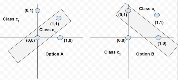
So, any point (x,₁x₂) which lies above the decision boundary, as depicted by the graph, will be assigned to class c1 and the points which lie below the boundary are assigned to class c2. 

Thus, we see that for a data set with linearly separable classes, perceptrons can always be employed to solve classification problems using decision lines (for 2-dimensional space), decision planes (for 3-dimensional space) or decision hyperplanes (for n-dimensional space). Appropriate values of the synaptic weights can be obtained by training a perceptron. However, one assumption for perceptron to work properly is that the two classes should be linearly separable i.e. the classes should be sufficiently separated from each other. Otherwise, if the classes are non-linearly separable, then the classification problem cannot be solved by perceptron.

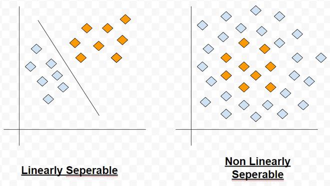
Linear Vs Non-Linearly Separable Classes

Multi-layer perceptron: A basic perceptron works very successfully for data sets which possess linearly separable patterns. However, in practical situations, that is an ideal situation to have. This was exactly the point driven by Minsky and Papert in their work in 1969. They showed that a basic perceptron is not able to learn to compute even a simple 2 bit XOR. So, let us understand the reason. 

Consider a truth table highlighting output of a 2 bit XOR function:

x1	x2	x1 XOR x2	Class
1	1	0	c2
1	0	1	c1
0	1	1	c1
0	0	0	c2

The data is not linearly separable. Only a curved decision boundary can separate the classes properly. To address this issue, the other option is to use two decision boundary lines in place of one. 

Classification with two decision lines in the XOR function output

This is the philosophy used to design the multi-layer perceptron model. The major highlights of this model are as follows:

• The neural network contains one or more intermediate layers between the input and output nodes, which are hidden from both input and output nodes
• Each neuron in the network includes a non-linear activation function that is differentiable.
• The neurons in each layer are connected with some or all the neurons in the previous layer.

3. ADALINE Network Model

Adaptive Linear Neural Element (ADALINE) is an early single-layer ANN developed by Professor Bernard Widrow of Stanford University. As depicted in the below diagram, it has only output neurons. The output value can be +1 or -1. A bias input x₀ (where x₀ =1) having a weight w₀ is added. The activation function is such that if weighted sum is positive or 0, the output is 1, else it is -1. Formally I can say that,

[Tex]y_{sum} = \sum_{i=1}^nw_ix_i+b, where\:b = w_0 [/Tex]

[Tex]y_{out}=f(y_{sum})=\bigg\{\begin{matrix} 1, x \geq 1 \\ -1, x < 1 \end{matrix} [/Tex]

The supervised learning algorithm adopted by ADALINE network is known as Least Mean Square (LMS) or DELTA Rule. A network combining a number of ADALINE is termed as MADALINE (many ADALINE). MEADALINE networks can be used to solve problems related to non-linear separability.