Implementation of Locally Weighted Linear Regression

LOESS or LOWESS are non-parametric regression methods that combine multiple regression models in a k-nearest-neighbor-based meta-model. LOESS combines much of the simplicity of linear least squares regression with the flexibility of nonlinear regression. It does this by fitting simple models to localized subsets of the data to build up a function that describes the variation in the data, point by point. 

• This algorithm is used for making predictions when there exists a non-linear relationship between the features.
• Locally weighted linear regression is a supervised learning algorithm.
• It a non-parametric algorithm.
• doneThere exists No training phase. All the work is done during the testing phase/while making predictions.

Suppose we want to evaluate the hypothesis function h at a certain query point x. For linear regression we would do the following: 



For locally weighted linear regression we will instead do the following: 




where w(i) is a is a non-negative “weight” associated with training point x(i). A higher “preference” is given to the points in the training set lying in the vicinity of x than the points lying far away from x. so For x(i) lying closer to the query point x, the value of w(i) is large, while for x(i) lying far away from x the value of w(i) is small. 
w(i) can be chosen as – 

Directly using closed Form solution to find parameters- 

Code: Importing Libraries :

python

import numpy as np
import matplotlib.pyplot as plt
import pandas as pd

plt.style.use("seaborn")

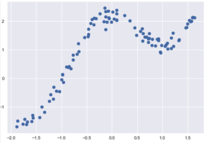
Code: Loading Data :

python

# Loading CSV files from local storage
dfx = pd.read_csv('weightedX_LOWES.csv')
dfy = pd.read_csv('weightedY_LOWES.csv')
# Getting data from DataFrame Object and storing in numpy n-dim arrays
X = dfx.values
Y = dfy.values

Output: 

Code: Function to calculate weight matrix :

python

# function to calculate W weight diagonal Matrix used in calculation of predictions
def get_WeightMatrix_for_LOWES(query_point, Training_examples, Bandwidth):
  # M is the No of training examples
  M = Training_examples.shape[0]
  # Initialising W with identity matrix
  W = np.mat(np.eye(M))
  # calculating weights for query points
  for i in range(M):
    xi = Training_examples[i]
    denominator = (-2 * Bandwidth * Bandwidth)
    W[i, i] = np.exp(np.dot((xi-query_point), (xi-query_point).T)/denominator)
    return W

Code: Making Predictions:

python

# function to make predictions
def predict(training_examples, Y, query_x, Bandwidth):
  M = Training_examples.shape[0]
  all_ones = np.ones((M, 1))
  X_ = np.hstack((training_examples, all_ones))
  qx = np.mat([query_x, 1])
  W = get_WeightMatrix_for_LOWES(qx, X_, Bandwidth)
  # calculating parameter theta
  theta = np.linalg.pinv(X_.T*(W * X_))*(X_.T*(W * Y))
  # calculating predictions
  pred = np.dot(qx, theta)
  return theta, pred

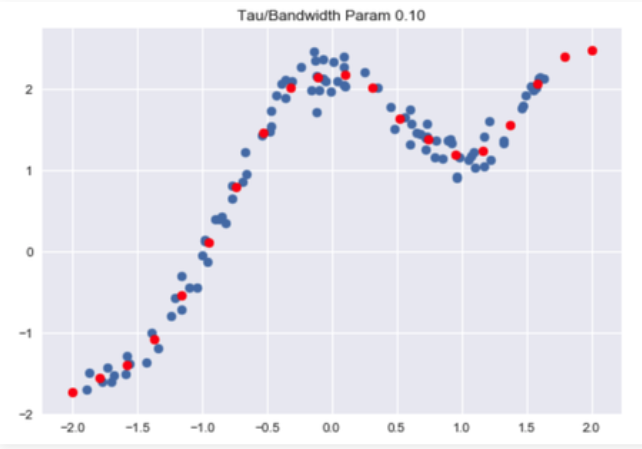
Code: Visualise Predictions :

python

# visualise predicted values with respect
# to original target values

Bandwidth = 0.1
X_test = np.linspace(-2, 2, 20)
Y_test = []
for query in X_test:
  theta, pred = predict(X, Y, query, Bandwidth)
  Y_test.append(pred[0][0])
horizontal_axis = np.array(X)
vertical_axis = np.array(Y)
plt.title("Tau / Bandwidth Param %.2f"% Bandwidth)
plt.scatter(horizontal_axis, vertical_axis)
Y_test = np.array(Y_test)
plt.scatter(X_test, Y_test, color ='red')
plt.show()