Implementation of Bayesian Regression

Last Updated : 28 Jan, 2024

Linear regression is a popular regression approach in machine learning. Linear regression is based on the assumption that the underlying data is normally distributed and that all relevant predictor variables have a linear relationship with the outcome. But In the real world, this is not always possible, it will follows these assumptions, Bayesian regression could be the better choice.
Bayesian regression employs prior belief or knowledge about the data to “learn” more about it and create more accurate predictions. It also takes into account the data’s uncertainty and leverages prior knowledge to provide more precise estimates of the data. As a result, it is an ideal choice when the data is complex or ambiguous.

Bayesian regression uses a Bayes algorithm to estimate the parameters of a linear regression model from data, including prior knowledge about the parameters. Because of its probabilistic character, it can produce more accurate estimates for regression parameters than ordinary least squares (OLS) linear regression, provide a measure of uncertainty in the estimation, and make stronger conclusions than OLS. Bayesian regression can also be utilized for related regression analysis tasks like model selection and outlier detection.

Bayesian Regression

Bayesian regression is a type of linear regression that uses Bayesian statistics to estimate the unknown parameters of a model. It uses Bayes’ theorem to estimate the likelihood of a set of parameters given observed data. The goal of Bayesian regression is to find the best estimate of the parameters of a linear model that describes the relationship between the independent and the dependent variables.

The main difference between traditional linear regression and Bayesian regression is the underlying assumption regarding the data-generating process. Traditional linear regression assumes that data follows a Gaussian or normal distribution, while Bayesian regression has stronger assumptions about the nature of the data and puts a prior probability distribution on the parameters. Bayesian regression also enables more flexibility as it allows for additional parameters or prior distributions, and can be used to construct an arbitrarily complex model that explicitly expresses prior beliefs about the data. Additionally, Bayesian regression provides more accurate predictive measures from fewer data points and is able to construct estimates for uncertainty around the estimates. On the other hand, traditional linear regressions are easier to implement and generally faster with simpler models and can provide good results when the assumptions about the data are valid.

Bayesian Regression can be very useful when we have insufficient data in the dataset or the data is poorly distributed. The output of a Bayesian Regression model is obtained from a probability distribution, as compared to regular regression techniques where the output is just obtained from a single value of each attribute.

Some Dependent Concepts for Bayesian Regression

The important concepts in Bayesian Regression are as follows:

Bayes Theorem

Bayes Theorem gives the relationship between an event’s prior probability and its posterior probability after evidence is taken into account. It states that the conditional probability of an event is equal to the probability of the event given certain conditions multiplied by the prior probability of the event, divided by the probability of the conditions.
i.e $P(A | B) = \frac{P(B | A) \cdot P(A)} {P(B)}$ .
Where P(A|B) is the probability of event A occurring given that event B has already occurred, P(B|A) is the probability of event B occurring given that event A has already occurred, P(A) is the probability of event A occurring and P(B) is the probability of event B occurring.

Maximum Likelihood Estimation (MLE)

MLE is a method used to estimate the parameters of a statistical model by maximizing the likelihood function. it seeks to find the parameter values that make the observed data most probable under the assumed model. MLE does not incorporate any prior information or assumptions about the parameters, and it provides point estimates of the parameters

Maximum A Posteriori (MAP) Estimation

MAP estimation is a Bayesian approach that combines prior information with the likelihood function to estimate the parameters. It involves finding the parameter values that maximize the posterior distribution, which is obtained by applying Bayes’ theorem. In MAP estimation, a prior distribution is specified for the parameters, representing prior beliefs or knowledge about their values. The likelihood function is then multiplied by the prior distribution to obtain the joint distribution, and the parameter values that maximize this joint distribution are selected as the MAP estimates. MAP estimation provides point estimates of the parameters, similar to MLE, but incorporates prior information.

Need for Bayesian Regression

There are several reasons why Bayesian regression is useful over other regression techniques. Some of them are as follows:

Bayesian regression also uses the prior belief about the parameters in the analysis. which makes it useful when there is limited data available and the prior knowledge are relevant. By combining prior knowledge with the observed data, Bayesian regression provides more informed and potentially more accurate estimates of the regression parameters.
Bayesian regression provides a natural way to measure the uncertainty in the estimation of regression parameters by generating the posterior distribution, which captures the uncertainty in the parameter values, as opposed to the single point estimate that is produced by standard regression techniques. This distribution offers a range of acceptable values for the parameters and can be used to compute trustworthy intervals or Bayesian confidence intervals.
In order to incorporate complicated correlations and non-linearities, Bayesian regression provides flexibility by offering a framework for integrating various prior distributions, which makes it capable to handle situations where the basic assumptions of standard regression techniques, like linearity or homoscedasticity, may not be true. It enables the modeling of more realistic and nuanced relationships between the predictors and the response variable.
Bayesian regression facilitates model selection and comparison by calculating the posterior probabilities of different models.
Bayesian regression can handle outliers and influential observations more effectively compared to classical regression methods. It provides a more robust approach to regression analysis, as extreme or influential observations have a lesser impact on the estimation.

Implementation of Bayesian Regression

Let’s independent features for linear regression is $X = \{x_1, x_2, ..., x_P\}$ , where xᵢ represents the i^th independent features and target variables will be Y. Assume we have n samples of (X, y)
The linear relationship between the dependent variable Y and the independent features X can be represented as:

$y = w_₀ + w_₁x_₁ + w_₂x_₂ + ... + w_ₚx_ₚ + \epsilon$
or
$y = f(x,w) + \epsilon$

Here, $w = \{w_₀, w_₁, w_₂, ..., w_ₚ\}$ are the regression coefficients, representing the relationship between the independent variables and the dependent variable, and ε is the error term.

We assume that the errors (ε) follow a normal distribution with mean 0 and constant variance $\sigma^2$ i.e. $(\epsilon \sim N(0, \sigma^2))$ . This assumption allows us to model the distribution of the target variable around the predicted values.

Likelihood Function

The probability distribution that builds the relationship between the independent features and the regression coefficients is known as likehood. It describes the probability of obtaining a certain result given some combination of regression coefficients.

Assumptions:

The errors $\epsilon = \{\epsilon_1, \epsilon_₂, ..., \epsilon_ₙ\}$ are independent and identical and follow a normal distribution with mean 0 and variance σ².

This means the target variable Y, given the predictor X₁, X₂, …, X_p follows a normal distribution with mean $\mu = f(x,w) = w_0 + w_1x_1 + w_2x_2 + ... + w_px_p$ and variance $\sigma^2$ .
Therefore, The conditional probability density function (PDF) of Y given the predictor variables will be:

$\begin{aligned} P(y|x,w,\sigma^2) &= N(f(x,w),\sigma^2) \\&=\frac{1}{\sqrt{2\pi\sigma^2}}e^{\left[-\frac{(y -f(x,w))^{2}}{2\sigma^{2}}\right]} \\&=\frac{1}{\sqrt{2\pi\sigma^2}}\exp{\left[\frac{y-(w_0+w_1x_{1}+w_2x_{2}+\cdots +w_P x_{P})}{2\sigma^2}\right]} \end{aligned}$

The likelihood function, for the n observations having each observation $(x_{i1}, x_{i2}, \cdots, x_{iP}, yᵢ)$ that follows a normal distribution with mean $\mu_i = w_{0} + w_1x_{i1} + w_2x_{i2} + \cdots + w_{P}x_{iP}$ and variance $\sigma^2$ , will be the joint probability density function (PDF) of the dependent variables, and can be written as the product of the individual PDFs::

$\begin{aligned} L(Y|X,w,\sigma^2) &= P(y_1 | x_{11}, x_{12},\cdots, x_{1P}) \cdot P(y_2 | x_{21}, x_{22},\cdots, x_{2P})\cdots P(y_n | x_{n1}, x_{n2},\cdots, x_{nP}) \\ &= N(f(x_{1p},w),\sigma^{2})\cdot N(f(x_{2p},w),\sigma^{2}) \cdots N(f(x_{np},w),\sigma^{2})\cdot \\& = \prod_{i=1}^{N}[N(f(x_{ip},w),\sigma^{2})] \end{aligned}$

To simplify calculations, we can take the logarithm of the likelihood function:

$\begin{aligned} \ln(L(Y|X,w,\sigma^2)) &= \ln{\left[ \prod_{i=1}^{N}[N(f(x_{ip},w),\sigma^{2})]\right ]} \\&= \ln{[N(f(x_{1p},w),\sigma^{2})}] + \ln[N(f(x_{2p},w),\sigma^{2})] + \cdots + \ln{[N(f(x_{np},w),\sigma^{2})]} \\&=\sum_{i=1}^{N}\ln\left[ \frac{1}{\sqrt{2\pi\sigma^2}} \exp\left(-\frac{(y_i-(w_0+w_1x_{i1}+w_2x_{i2}+\cdots +w_P x_{iP}))^2}{2\sigma^2}\right) \right] \end{aligned}$

Precision:

\beta = \frac{1}{\sigma^2}

Using the conditional PDF expression from the previous response, we substitute it into the likelihood function:

$\ln(L(y|x,w,\sigma^2))= \frac{N}{2}\ln(2\pi)-\frac{N}{2}\ln(\beta)-\frac{\beta}{2}\sum_{i=1}^{N}\left[(y-f(x_i,w))^2 \right ]$

Negative Log likelihood

$-\ln(L(y|x,w,\sigma^2))= \frac{\beta}{2}\sum_{i=1}^{N}\left[(y-f(x_i,w))^2 \right ]-\frac{N}{2}\ln(2\pi)+\frac{N}{2}\ln(\beta)$

Here, $\ln(2\pi)$ and $\ln(\beta)$ are constant, So,

$-\ln(L(y|x,w,\sigma^2))= \frac{\beta}{2}\sum_{i=1}^{N}\left[(y-f(x_i,w))^2 \right ] + \text{constant}$

Prior:

Prior is the initial belief or probability about the parameter before observing the data. It is the information or assumption about the parameters.
In Maximum A Posteriori (MAP) estimation, we incorporate prior knowledge or beliefs about the parameters into the estimation process. We represent this prior information using a prior distribution, denoted by P(w|\alpha) =N(0,\alpha^{-1}I)

Posterior Distribution:

The posterior distribution is the updated beliefs or probability distribution of parameters, which comes after taking into account the prior distribution of parameters and the observed data.
Using Bayes’ theorem, we can express the posterior distribution in terms of the likelihood function and the prior distribution:

$P(w|X,\alpha, \beta^{-1}) = \frac{L(Y|X,w, \beta^{-1}) \cdot P(w|\alpha)}{P(Y|X)}$

P(Y|X) is the marginal probability of the observed data, which acts as a normalizing constant. Since it does not depend on the parameter values, we can ignore it in the optimization process.

$P(w | X,\alpha, \beta^{-1}) \propto(L(Y|X,w, \beta^{-1}) \cdot P(w|\alpha))$

In the above formula,

Log-likelihood : $L(Y|X, w, \beta^{-1})$ is normal distribution
Prior : $P(w|\alpha)$ is uniform
So, the Posterior will also be the normal distribution.

In practice, it is often more convenient to work with the log of the posterior distribution, known as the log-posterior:

For getting maximum posterior distribution, we use the negative likelihood

$\begin{aligned} \hat{w}&= \ln[(L(Y|X,w, \beta^{-1}) \cdot P(w|\alpha))] \\ &= \ln[L(Y|X,w, \beta^{-1})] + \ln[P(w|\alpha)] \\&=\frac{ \beta}{2}\sum_{i=1}^{N}(y_i-f(xᵢ,w))² + \frac{\alpha}{2} w^T w \end{aligned}$

Maximum of Posterior is given by a minimum of $\frac{ \beta}{2}\sum_{i=1}^{N}(y_i-f(xᵢ,w))² + \frac{\alpha}{2} w^T w$

Implementation of Bayesian Regression Using Python:

Method 1:

Python3

#Import the necessary libraries
import torch
import pyro
import pyro.distributions as dist
from pyro.infer import SVI, Trace_ELBO, Predictive
from pyro.optim import Adam
import matplotlib.pyplot as plt
import seaborn as sns
 
 
# Generate some sample data
torch.manual_seed(0)
X = torch.linspace(0, 10, 100)
true_slope = 2
true_intercept = 1
Y = true_intercept + true_slope * X + torch.randn(100)
 
# Define the Bayesian regression model
def model(X, Y):
    # Priors for the parameters
    slope = pyro.sample("slope", dist.Normal(0, 10))
    intercept = pyro.sample("intercept", dist.Normal(0, 10))
    sigma = pyro.sample("sigma", dist.HalfNormal(1))
 
    # Expected value of the outcome
    mu = intercept + slope * X
 
    # Likelihood (sampling distribution) of the observations
    with pyro.plate("data", len(X)):
        pyro.sample("obs", dist.Normal(mu, sigma), obs=Y)
 
# Run Bayesian inference using SVI (Stochastic Variational Inference)
def guide(X, Y):
    # Approximate posterior distributions for the parameters
    slope_loc = pyro.param("slope_loc", torch.tensor(0.0))
    slope_scale = pyro.param("slope_scale", torch.tensor(1.0),
                             constraint=dist.constraints.positive)
    intercept_loc = pyro.param("intercept_loc", torch.tensor(0.0))
    intercept_scale = pyro.param("intercept_scale", torch.tensor(1.0),
                                 constraint=dist.constraints.positive)
    sigma_loc = pyro.param("sigma_loc", torch.tensor(1.0), 
                           constraint=dist.constraints.positive)
 
    # Sample from the approximate posterior distributions
    slope = pyro.sample("slope", dist.Normal(slope_loc, slope_scale))
    intercept = pyro.sample("intercept", dist.Normal(intercept_loc, 
                                                     intercept_scale))
    sigma = pyro.sample("sigma", dist.HalfNormal(sigma_loc))
 
# Initialize the SVI and optimizer
optim = Adam({"lr": 0.01})
svi = SVI(model, guide, optim, loss=Trace_ELBO())
 
# Run the inference loop
num_iterations = 1000
for i in range(num_iterations):
    loss = svi.step(X, Y)
    if (i + 1) % 100 == 0:
        print(f"Iteration {i + 1}/{num_iterations} - Loss: {loss}")
 
# Obtain posterior samples using Predictive
predictive = Predictive(model, guide=guide, num_samples=1000)
posterior = predictive(X, Y)
 
# Extract the parameter samples
slope_samples = posterior["slope"]
intercept_samples = posterior["intercept"]
sigma_samples = posterior["sigma"]
 
# Compute the posterior means
slope_mean = slope_samples.mean()
intercept_mean = intercept_samples.mean()
sigma_mean = sigma_samples.mean()
 
# Print the estimated parameters
print("Estimated Slope:", slope_mean.item())
print("Estimated Intercept:", intercept_mean.item())
print("Estimated Sigma:", sigma_mean.item())
 
 
# Create subplots
fig, axs = plt.subplots(1, 3, figsize=(15, 5))
 
# Plot the posterior distribution of the slope
sns.kdeplot(slope_samples, shade=True, ax=axs[0])
axs[0].set_title("Posterior Distribution of Slope")
axs[0].set_xlabel("Slope")
axs[0].set_ylabel("Density")
 
# Plot the posterior distribution of the intercept
sns.kdeplot(intercept_samples, shade=True, ax=axs[1])
axs[1].set_title("Posterior Distribution of Intercept")
axs[1].set_xlabel("Intercept")
axs[1].set_ylabel("Density")
 
# Plot the posterior distribution of sigma
sns.kdeplot(sigma_samples, shade=True, ax=axs[2])
axs[2].set_title("Posterior Distribution of Sigma")
axs[2].set_xlabel("Sigma")
axs[2].set_ylabel("Density")
 
# Adjust the layout
plt.tight_layout()
 
# Show the plot
plt.show()

Output:

Iteration 100/1000 - Loss: 26402.827576458454
Iteration 200/1000 - Loss: 868.8797441720963
Iteration 300/1000 - Loss: 375.8896267414093
Iteration 400/1000 - Loss: 410.9912616610527
Iteration 500/1000 - Loss: 1326.6764334440231
Iteration 600/1000 - Loss: 6281.599338412285
Iteration 700/1000 - Loss: 928.897826552391
Iteration 800/1000 - Loss: 162330.28921669722
Iteration 900/1000 - Loss: 803.6285791993141
Iteration 1000/1000 - Loss: 16296.759144246578
Estimated Slope: 0.6329146027565002
Estimated Intercept: 0.632161021232605
Estimated Sigma: 1.5464321374893188

Posterior Distribution of Parameters-Geeksforgeeks

Method:2

Python3

import numpy as np
import pymc3 as pm
import matplotlib.pyplot as plt
 
# Generate some sample data
np.random.seed(0)
X = np.linspace(0, 10, 100)
true_slope = 2
true_intercept = 1
Y = true_intercept + true_slope * X + np.random.normal(0, 1, size=100)
 
# Create a PyMC3 model
with pm.Model() as model:
    # Priors for the parameters
    slope = pm.Normal('slope', mu=0, sd=10)
    intercept = pm.Normal('intercept', mu=0, sd=10)
    sigma = pm.HalfNormal('sigma', sd=1)
 
    # Expected value of the outcome
    mu = intercept + slope * X
 
    # Likelihood (sampling distribution) of the observations
    Y_obs = pm.Normal('Y_obs', mu=mu, sd=sigma, observed=Y)
 
    # Run the MCMC sampling
    trace = pm.sample(2000, tune=1000)
 
# Plot the posterior distributions
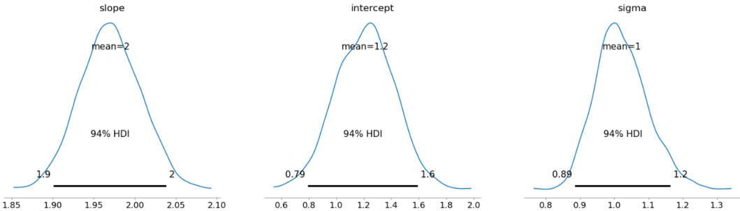
pm.plot_posterior(trace, var_names=['slope', 'intercept', 'sigma'])
plt.show()

Output:

 100.00% [6000/6000 00:02<00:00 Sampling 2 chains, 0 divergences]

Posterior Distributions of the Parameters-Geeksforgeeks

Advantages of Bayesian Regression:

Very effective when the size of the dataset is small.
Particularly well-suited for on-line based learning (data is received in real-time), as compared to batch-based learning, where we have the entire dataset on our hands before we start training the model. This is because Bayesian Regression doesn’t need to store data.
The Bayesian approach is a tried and tested approach and is very robust, mathematically. So, one can use this without having any extra prior knowledge about the dataset.
Bayesian regression methods employ skewed distributions that let you include outside information in your model.

Disadvantages of Bayesian Regression:

The inference of the model can be time-consuming.
If there is a large amount of data available for our dataset, the Bayesian approach is not worth it and the regular frequentist approach does a more efficient job
If your code is in a setting where installing new packages is challenging and there are strong dependency controls, this might be an issue.
Many of the basic mistakes that commonly plague traditional frequentist regression models still apply to Bayesian models. For instance, Bayesian models still depend on the linearity of the relationship between the characteristics and the outcome variable.

When to use Bayesian Regression:

Small sample size: When you have a tiny sample size, Bayesian inference is frequently quite helpful. Bayesian regression is a wonderful choice if you need to develop a very complicated model but do not have access to a lot of data. In fact, it’s probably the greatest choice you have! Large sample sizes are necessary for many other machine-learning models to work properly.
Strong prior knowledge: The easiest method to include strong external knowledge into your model is by utilising a Bayesian model. The influence of the prior knowledge will be more obvious the smaller the dataset size you work with.

Conclusion:

So now that you know how Bayesian regressors work and when to use them, you should try using it next time you want to perform a regression task, especially if the dataset is small.

Suggest improvement

Polynomial Regression ( From Scratch using Python )

How to Perform Quantile Regression in Python

Share your thoughts in the comments

Getting Started with Machine Learning

Data Preprocessing

Classification & Regression

K-Nearest Neighbors (KNN)

Support Vector Machines

Decision Tree

Ensemble Learning

Generative Model

Time Series Forecasting

Clustering Algorithm

Convolutional Neural Networks

Recurrent Neural Networks

Reinforcement Learning

Model Deployment and Productionization

Advanced Topics

Getting Started with Machine Learning

Data Preprocessing

Classification & Regression

K-Nearest Neighbors (KNN)

Support Vector Machines

Decision Tree

Ensemble Learning

Generative Model

Time Series Forecasting

Clustering Algorithm

Convolutional Neural Networks

Recurrent Neural Networks

Reinforcement Learning

Model Deployment and Productionization

Advanced Topics

Implementation of Bayesian Regression

Bayesian Regression

Some Dependent Concepts for Bayesian Regression

Bayes Theorem

Maximum Likelihood Estimation (MLE)

Maximum A Posteriori (MAP) Estimation

Need for Bayesian Regression

Implementation of Bayesian Regression

Likelihood Function

Assumptions:

Negative Log likelihood

Prior:

Posterior Distribution:

Implementation of Bayesian Regression Using Python:

Method 1:

Python3

Method:2

Python3

Advantages of Bayesian Regression:

Disadvantages of Bayesian Regression:

When to use Bayesian Regression:

Conclusion:

Please Login to comment...

Similar Reads

What kind of Experience do you want to share?