Implementation of a CNN based Image Classifier using PyTorch

Introduction:

Introduced in the 1980s by Yann LeCun, Convolution Neural Networks(also called CNNs or ConvNets) have come a long way. From being employed for simple digit classification tasks, CNN-based architectures are being used very profoundly over much Deep Learning and Computer Vision-related tasks like object detection, image segmentation, gaze tracking, among others. Using the PyTorch framework, this article will implement a CNN-based image classifier on the popular CIFAR-10 dataset. 

Before going ahead with the code and installation, the reader is expected to understand how CNNs work theoretically and with various related operations like convolution, pooling, etc. The article also assumes a basic familiarity with the PyTorch workflow and its various utilities, like Dataloaders, Datasets, Tensor transforms, and CUDA operations. For a quick refresher of these concepts, the reader is encouraged to go through the following articles:

• Introduction to Convolutional Neural Network
• Training Neural Networks with Validation using PyTorch
• How to set up and Run CUDA Operations in Pytorch?

Installation

For the implementation of the CNN and downloading the CIFAR-10 dataset, we’ll be requiring the torch and torchvision modules. Apart from that, we’ll be using numpy and matplotlib for data analysis and plotting. The required libraries can be installed using the pip package manager through the following command:

    pip install torch torchvision torchaudio numpy matplotlib

Stepwise implementation

Step 1: Downloading data and printing some sample images from the training set.

• Before starting our journey to implementing CNN, we first need to download the dataset onto our local machine, which we’ll be training our model over. We’ll be using the torchvision utility for this purpose and downloading the CIFAR-10 dataset into training and testing sets in directories “./CIFAR10/train” and “./CIFAR10/test,“ respectively. We also apply a normalized transform where the procedure is done over the three channels for all the images.
• Now, we have a training dataset and a test dataset with 50000 and 10000 images, respectively, of a dimension 32x32x3. After that, we convert these datasets into data loaders of a batch size of 128 for better generalization and a faster training process.
• Finally, we plot out some sample images from the 1st training batch to get an idea of the images we’re dealing with using the make_grid utility from torchvision.

Code:

Python3

import torch
import torchvision
import matplotlib.pyplot as plt
import numpy as np

# The below two lines are optional and are just there to avoid any SSL
# related errors while downloading the CIFAR-10 dataset
import ssl
ssl._create_default_https_context = ssl._create_unverified_context

#Defining plotting settings
plt.rcParams['figure.figsize'] = 14, 6

#Initializing normalizing transform for the dataset
normalize_transform = torchvision.transforms.Compose([
    torchvision.transforms.ToTensor(),
    torchvision.transforms.Normalize(mean = (0.5, 0.5, 0.5),
                                     std = (0.5, 0.5, 0.5))])

#Downloading the CIFAR10 dataset into train and test sets
train_dataset = torchvision.datasets.CIFAR10(
    root="./CIFAR10/train", train=True,
    transform=normalize_transform,
    download=True)

test_dataset = torchvision.datasets.CIFAR10(
    root="./CIFAR10/test", train=False,
    transform=normalize_transform,
    download=True)

#Generating data loaders from the corresponding datasets
batch_size = 128
train_loader = torch.utils.data.DataLoader(train_dataset, batch_size=batch_size)
test_loader = torch.utils.data.DataLoader(test_dataset, batch_size=batch_size)

#Plotting 25 images from the 1st batch
dataiter = iter(train_loader)
images, labels = dataiter.next()
plt.imshow(np.transpose(torchvision.utils.make_grid(
  images[:25], normalize=True, padding=1, nrow=5).numpy(), (1, 2, 0)))
plt.axis('off')

Output:

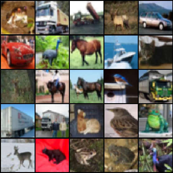
Figure 1: Some sample images from the training dataset

Step-2: Plotting class distribution of the dataset

It’s generally a good idea to plot out the class distribution of the training set. This helps in checking whether the provided dataset is balanced or not. To do this, we iterate over the entire training set in batches and collect the respective classes of each instance. Finally, we calculate the counts of the unique classes and plot them.

Code:

Python3

#Iterating over the training dataset and storing the target class for each sample
classes = []
for batch_idx, data in enumerate(train_loader, 0):
    x, y = data
    classes.extend(y.tolist())

#Calculating the unique classes and the respective counts and plotting them
unique, counts = np.unique(classes, return_counts=True)
names = list(test_dataset.class_to_idx.keys())
plt.bar(names, counts)
plt.xlabel("Target Classes")
plt.ylabel("Number of training instances")

Output:

Figure 2: Class distribution of the training set

As shown in Figure 2, each of the ten classes has almost the same number of training samples. Thus we don’t need to take additional steps to rebalance the dataset.

Step-3: Implementing the CNN architecture

On the architecture side, we’ll be using a simple model that employs three convolution layers with depths 32, 64, and 64, respectively, followed by two fully connected layers for performing classification. 

• Each convolutional layer involves a convolutional operation involving a 3×3 convolution filter and is followed by a ReLU activation operation for introducing nonlinearity into the system and a max-pooling operation with a 2×2 filter to reduce the dimensionality of the feature map.
• After the end of the convolutional blocks, we flatten the multidimensional layer into a low dimensional structure for starting our classification blocks. After the first linear layer, the last output layer(also a linear layer) has ten neurons for each of the ten unique classes in our dataset.

The architecture is as follows:

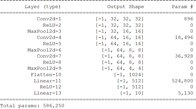
Figure 3: Architecture of the CNN

For building our model, we’ll make a CNN class inherited from the torch.nn.Module class for taking advantage of the Pytorch utilities. Apart from that, we’ll be using the torch.nn.Sequential container to combine our layers one after the other. 

• The Conv2D(), ReLU(), and MaxPool2D() layers perform the convolution, activation, and pooling operations. We used padding of 1 to give sufficient learning space to the kernel as padding gives the image more coverage area, especially the pixels in the outer frame.
• After the convolutional blocks, the Linear() fully connected layers perform classification.

Code:

Python3

class CNN(torch.nn.Module):
    def __init__(self):
        super().__init__()
        self.model = torch.nn.Sequential(
            #Input = 3 x 32 x 32, Output = 32 x 32 x 32
            torch.nn.Conv2d(in_channels = 3, out_channels = 32, kernel_size = 3, padding = 1),
            torch.nn.ReLU(),
            #Input = 32 x 32 x 32, Output = 32 x 16 x 16
            torch.nn.MaxPool2d(kernel_size=2),

            #Input = 32 x 16 x 16, Output = 64 x 16 x 16
            torch.nn.Conv2d(in_channels = 32, out_channels = 64, kernel_size = 3, padding = 1),
            torch.nn.ReLU(),
            #Input = 64 x 16 x 16, Output = 64 x 8 x 8
            torch.nn.MaxPool2d(kernel_size=2),

            #Input = 64 x 8 x 8, Output = 64 x 8 x 8
            torch.nn.Conv2d(in_channels = 64, out_channels = 64, kernel_size = 3, padding = 1),
            torch.nn.ReLU(),
            #Input = 64 x 8 x 8, Output = 64 x 4 x 4
            torch.nn.MaxPool2d(kernel_size=2),

            torch.nn.Flatten(),
            torch.nn.Linear(64*4*4, 512),
            torch.nn.ReLU(),
            torch.nn.Linear(512, 10)
        )

    def forward(self, x):
        return self.model(x)

Step-4: Defining the training parameters and beginning the training process

We begin the training process by selecting the device to train our model onto, i.e., CPU or a GPU. Then, we define our model hyperparameters which are as follows:

• We train our models over 50 epochs, and since we have a multiclass problem, we used the Cross-Entropy Loss as our objective function.
• We used the popular Adam optimizer with a learning rate of 0.001 and weight_decay of 0.01 to prevent overfitting through regularization to optimize the objective function.

Finally, we begin our training loop, which involves calculating outputs for each batch and the loss by comparing the predicted labels with the true labels. In the end, we’ve plotted the training loss for each respective epoch to ensure the training process went as per the plan.

Code:

Python3

#Selecting the appropriate training device
device = 'cuda' if torch.cuda.is_available() else 'cpu'
model = CNN().to(device)

#Defining the model hyper parameters
num_epochs = 50
learning_rate = 0.001
weight_decay = 0.01
criterion = torch.nn.CrossEntropyLoss()
optimizer = torch.optim.Adam(model.parameters(), lr=learning_rate, weight_decay=weight_decay)

#Training process begins
train_loss_list = []
for epoch in range(num_epochs):
    print(f'Epoch {epoch+1}/{num_epochs}:', end = ' ')
    train_loss = 0

    #Iterating over the training dataset in batches
    model.train()
    for i, (images, labels) in enumerate(train_loader):

        #Extracting images and target labels for the batch being iterated
        images = images.to(device)
        labels = labels.to(device)

        #Calculating the model output and the cross entropy loss
        outputs = model(images)
        loss = criterion(outputs, labels)

        #Updating weights according to calculated loss
        optimizer.zero_grad()
        loss.backward()
        optimizer.step()
        train_loss += loss.item()

    #Printing loss for each epoch
    train_loss_list.append(train_loss/len(train_loader))
    print(f"Training loss = {train_loss_list[-1]}")

#Plotting loss for all epochs
plt.plot(range(1,num_epochs+1), train_loss_list)
plt.xlabel("Number of epochs")
plt.ylabel("Training loss")

Output:

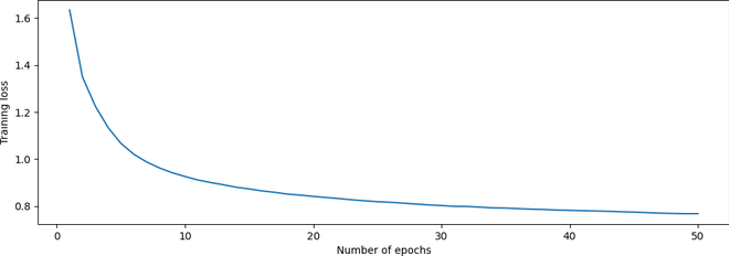
Figure 4: Plot of training loss vs. number of epochs

From FIgure 4, we can see that the loss decreases as the epochs increase, indicating a successful training procedure.

Step-5: Calculating the model’s accuracy on the test set

Now that our model’s trained, we need to check its performance on the test set. To do that, we iterate over the entire test set in batches and calculate the accuracy score by comparing the true and predicted labels for each batch. 

Code:

Python3

test_acc=0
model.eval()

with torch.no_grad():
    #Iterating over the training dataset in batches
    for i, (images, labels) in enumerate(test_loader):

        images = images.to(device)
        y_true = labels.to(device)

        #Calculating outputs for the batch being iterated
        outputs = model(images)

        #Calculated prediction labels from models
        _, y_pred = torch.max(outputs.data, 1)

        #Comparing predicted and true labels
        test_acc += (y_pred == y_true).sum().item()

    print(f"Test set accuracy = {100 * test_acc / len(test_dataset)} %")

Output:

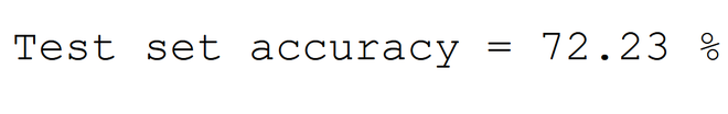
Figure 5: Accuracy on the test set

Step 6: Generating predictions for sample images in the test set

As shown in Figure 5, our model has achieved an accuracy of nearly 72%. To validate its performance, we can generate some predictions for some sample images. To do that, we take the first five images of the last batch of the test set and plot them using the make_grid utility from torchvision. We then collect their true labels and predictions from the model and show them in the plot’s title.

Code:

Python3

#Generating predictions for 'num_images' amount of images from the last batch of test set
num_images = 5
y_true_name = [names[y_true[idx]] for idx in range(num_images)]
y_pred_name = [names[y_pred[idx]] for idx in range(num_images)]

#Generating the title for the plot
title = f"Actual labels: {y_true_name}, Predicted labels: {y_pred_name}"

#Finally plotting the images with their actual and predicted labels in the title
plt.imshow(np.transpose(torchvision.utils.make_grid(images[:num_images].cpu(), normalize=True, padding=1).numpy(), (1, 2, 0)))
plt.title(title)
plt.axis("off")

Output:

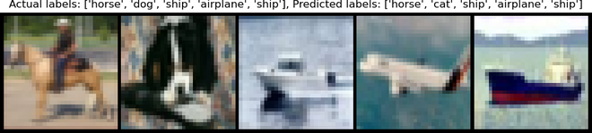
Figure 6: Actual vs. Predicted labels for 5 sample images from the test set. Note that the labels are in the same order as the respective images, from left to right.

As can be seen from Figure 6, the model is producing correct predictions for all the images except the 2nd one as it misclassifies the dog as a cat!

Conclusion:

This article covered the PyTorch implementation of a simple CNN on the popular CIFAR-10 dataset. The reader is encouraged to play around with the network architecture and model hyperparameters to increase the model accuracy even more!

References

1. https://cs231n.github.io/convolutional-networks/
2. https://pytorch.org/docs/stable/index.html
3. https://pytorch.org/tutorials/beginner/blitz/cifar10_tutorial.html