Implement Machine Learning With Caret In R

In today’s society, technological answers to human issues are knocking on the doors of practically all fields of knowledge. Every aspect of this universe’s daily operations generates data, and technology solutions base their decisions on these data-driven intuitions. In order to create a machine that learns from the obtained data and can address the aforementioned human problems, Machine Learning algorithms and approaches have emerged in this state. So, what exactly is Machine Learning?

A computer system that learns to do a task from data without being given instructions using mathematical and statistical models is known as Machine Learning. 

In this article, we’ll examine fundamental machine learning ideas, methods, and a step-by-step procedure of machine learning model developments by utilizing the R programming language’s Caret library.

Accordingly, there are two categories in which we may place machine learning algorithms: 

• Supervised learning:  It deals with labeled data or prediction purposes, 
• Unsupervised learning: It deals with unlabeled data or descriptive reasons. 

Depending on the goal and the available data, one may select one of these two algorithms.

Steps in Machine Learning using R

To get the intended outcomes, problems in data science must be decomposed into manageable tasks. We will walk through each step of implementing machine learning in R using the free and open-source Caret package in this part. The general steps to be followed in any Machine learning project are : 

• Data collection and importing
• Exploratory Data Analysis (EDA) 
• Data Preprocessing
• Model training and Evaluation

Let’s start the code.

Data collection and Importing

For modeling purposes, machine learning data should be gathered and imported into a R environment. These data sets may be electronically recorded on text or spreadsheets, SQL databases, or both. To begin your work, you must import the datasets into the R environment. However, in order to begin our task for this tutorial, we will import the data from the R dataset package. Install and import all prerequisite libraries that we will require for our project first.

The libraries are : 

• ggplot2 : It is used to interactive graphs and visualization.
• ggpubr : It is used to make our plot beautiful along with that of ggplot2.
• reshape : It is used to melt our dataset.
• caret: It is used to provide us with machine learning algorithms.

R

# To install packages
install.packages("ggplot2")
install.packages("ggpubr")
install.packages("reshape")
install.packages("caret")

After installing, let’s load the necessary packages.

R

# To load all necessary packages
library(ggplot2)
library(ggpubr)
library(reshape)
library(caret)

Next, we will import our data to a R environment.

R

# Dataset
data("iris")

# To display the first five
# rows of our data
head(iris)

Output:

We can use tail(iris) to see the bottom 5. If you want to see more than 5 rows, simply enter a number into the parentheses, e.g. head(iris, 10) or tail(iris, 10).

R

# To see the last five rows
# of our data
tail(iris)

Output:

Exploratory Data Analysis (EDA) 

Understanding and assessing the data you have for your project is one of the important steps in the modeling preparation process. This is accomplished through the use of data exploration, visualization, and statistical data summarization with a measure of central tendencies. You will gain an understanding of your data during this phase, and you will take a broad view of it to get ready for the modeling step. 

R

# Summary statistics of data
summary(iris)

Output:

R

# Visualizing the outliers by using boxplot
# As we use ggplot2 we will take numerical
# variables by subsetting the entire of it
df <- subset(iris, select = c(Sepal.Length,
                              Sepal.Width,
                              Petal.Length,
                              Petal.Width))

By using of reshape package we melt the data and plot it to check for the presence of any outliers. So, when we execute following code;

R

# plot and see the box plot of each variable
ggplot(data = melt(df),
       aes(x=variable, y=value)) +
        geom_boxplot(aes(fill=variable))

Output:

We can see that there is an outliers in the second column of the dataset.

R

# To plot the barplot for our
# categorical variable
ggplot(data = iris,
       aes(x = Species, fill = Species)) +
    geom_bar()

Output:

Let’s now use a histogram plot to visualize the distribution of our data’s continuous variables;

R

# In this we visualize the histogram of all
# numerical variables of the dataset
a <- ggplot(data = iris, aes(x = Petal.Length)) +
    geom_histogram( color = "red",
                   fill = "blue",
                   alpha = 0.01) + geom_density()

b <- ggplot(data = iris, aes(x = Petal.Width)) +
    geom_histogram( color = "red",
                   fill = "blue",
                   alpha = 0.1) + geom_density()
c <- ggplot(data = iris, aes(x = Sepal.Length)) +
    geom_histogram( color = "red",
                   fill = "blue",
                   alpha = 0.1) + geom_density()

d <- ggplot(data = iris, aes(x = Sepal.Width)) +
    geom_histogram( color = "red",
                   fill = "blue",
                   alpha = 0.1) +geom_density()

ggarrange(a, b, c, d + rremove("x.text"),
          labels = c("a", "b", "c", "d"),
          ncol = 2, nrow = 2)

Output : 

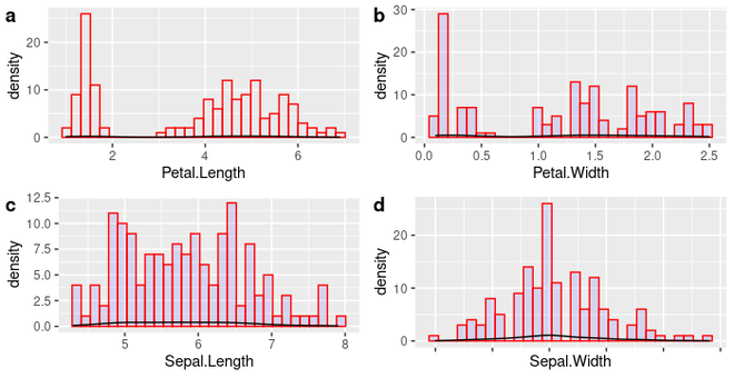
Histogram plot

Next, we will move to the Data Preparation phase of our machine learning process.  Before that, lets split our dataset into train, test and validation partition;

R

# Create train-test split of the data
limits <- createDataPartition(iris$Species,
                              p=0.80,
                              list=FALSE)

# select 20% of the data for validation
testiris <- iris[-limits,]

# use the remaining to training
# and testing the models
trainiris <- iris[limits,]

Data Preprocessing

The quality of our good predictions from the model depends on the quality of the data itself, making data preparation one of the most important steps in machine learning. The data and the work we want to do solely determine the time it takes, the method, and the process of purification and transformation of data into one of the relevant inputs. Here, we will examine how data preparation for our modeling is done.

We can see from the box plot that there are outliers in our data, and the histogram also shows how skewed the data is on the right and left sides. We shall thus eliminate those outliers from our data. 

R

Q <- quantile(trainiris$Sepal.Width,
              probs=c(.25, .75),
              na.rm = FALSE)

After obtaining the quantile value, we will additionally compute the interquartile range in order to determine the upper and lower bound cutoff values.

R

# Code to calculate the IQR,
# upper and lower bounds
iqr <- IQR(trainiris$Sepal.Width)
up <-  Q[2]+1.5*iqr
low<- Q[1]-1.5*iqr

Now, we can eliminate the outliers by using the below code.

R

# Elimination of outliers by using of iqr
normal <- subset(trainiris,
                 trainiris$Sepal.Width > (Q[1] - 1.5*iqr)
                 & trainiris$Sepal.Width < (Q[2]+1.5*iqr))
normal

Output : 

By using a boxplot, we can additionally see the outliers that were eliminated from the data.

R

# boxplot using cleaned dataset
boxes <- subset(normal,
                select = c(Sepal.Length,
                           Sepal.Width,
                           Petal.Length,
                           Petal.Width))
ggplot(data = melt(boxes),
       aes(x=variable, y=value)) +
        geom_boxplot(aes(fill=variable))

Output:

Model training and Evaluation

It’s time to use the prepared data to create a model. Since we don’t have a specific algorithm in mind, Let’s compare two machine learning methods for practical purposes and choose the one that performs the best;

• Linear Discriminant Analysis (LDA)
• Support Vector Machine (SVM)

For accuracy and prediction across all samples, we will employ 10-fold cross validation.

R

# crossvalidation set to 10
crossfold  <- trainControl(method="cv",
                           number=10,
                           savePredictions = TRUE)
metric <- "Accuracy"

Let’s start training model with Linear Discriminant Analysis.

R

# Set a random seed to 42
set.seed(42)
fit.lda <- train(Species~.,
                 data=trainiris,
                 method="lda",
                 metric=metric,
                 trControl=crossfold)
print(fit.lda)

Output : 

We can also use SVM model for the training. To train the Support Vector Machine, code is given below.

R

set.seed(42)
fit.svm <- train(Species~.,
                 data=trainiris,
                 method="svmRadial",
                 metric=metric,
                 trControl=crossfold)
print(fit.svm)

Output:

The results show that both algorithms functioned admirably with only minor variations. Although the model can be tuned to improve its accuracy accurate, for the purposes of this lesson, let’s stick with LDA and generate predictions using test data.

R

# prediction on test data
predictions <- predict(fit.lda, testiris)
confusionMatrix(predictions, testiris$Species)

Output : 

According to the summary of our model above, We see that the prediction performance is poor; this may be because we neglected to consider the LDA algorithm’s premise that the predictor variables should have the same variance, which is accomplished by scaling those features. We won’t deviate from the topic of this lesson because we are interested in developing machine learning utilizing the Caret module in R.

Conclusions

In conclusion, this is the most fundamental and entry-level introduction to the Caret library in R for machine learning. From here, you can begin working on your own project utilizing this straightforward introduction as a starting point.