Image Sharpening Using Laplacian Filter and High Boost Filtering in MATLAB

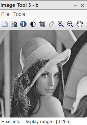
Image sharpening is an effect applied to digital images to give them a sharper appearance. Sharpening enhances the definition of edges in an image. The dull images are those which are poor at the edges. There is not much difference in background and edges. On the contrary, the sharpened image is that in which the edges are clearly distinguishable by the viewer. We know that intensity and contrast change at the edge. If this change is significant then the image is said to be sharp. The viewer can clearly see the background and foreground parts. 

Image sharpening using the smoothing technique

Laplacian Filter

• It is a second-order derivative operator/filter/mask. 
• It detects the image along with horizontal and vertical directions collectively. 
• There is no need to apply it separately to detect the edges along with horizontal and vertical directions. 
• The sum of the values of this filter is 0. 

Example:

Matlab

% MatLab program for edge sharpening.
% Read the image in variable 'a'
a=imread("cameraman.jpg");

% Defined the laplacian filter.
Lap=[0 1 0; 1 -4 1; 0 1 0];

% Convolve the image read
% in 'a' with Laplacian mask.
a1=conv2(a,Lap,'same');

% After convolution the intensity
% Values go beyond the range.
% Normalise the range of intensity.
a2=uint8(a1);

% Display the sharpened image.
imtool(abs(a-a2),[])

% Define strong laplacian filter
lap=[-1 -1 -1; -1 8 -1; -1 -1 -1];

% Apply filter on original image
a3=conv2(a,lap,'same');

% Normalise the resultant image.
a4=uint8(a3);

% Display the sharpened image.
imtool(abs(a+a4),[])

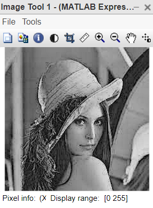
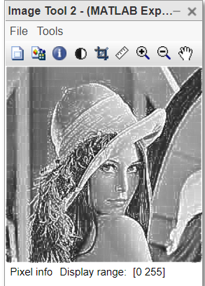
Output: 

Explanation of code:

• MatLab program explanation for edge sharpening. a=imread(“cameraman.jpg”); This line reads the image in variable a.
• Lap=[0 1 0; 1 -4 1; 0 1 0]; This line defines the Laplacian filter.
• a1=conv2(a Lap,’ same’); This line convolves the image with the Laplacian filter.
• After convolution, values of some pixels go beyond the range [0 255]. Hence the next line is used.
• a2=uint8(a1); This line normalizes the pixel range.
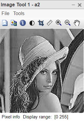
• Sharpened image = Original image – Edge detected image if the central pixel of Laplacian filter is a negative value.
• imtool(abs(a-a2),[]) This line displays the sharpened image.
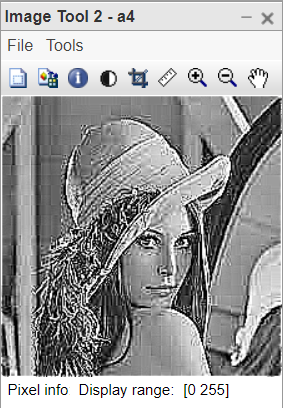
• lap=[-1 -1 -1; -1 8 -1; -1 -1 -1]; This line defines the strong Laplacian filter, with positive central pixel value.
• a3=conv2(a lap,’ same’); This line convolves the original image with this filter.
• a4=uint8(a3); This line normalizes the range of pixel values.
• imtool(abs(a+a4),[]) This line displays the sharpened image.

Using the sharpening mask: High Boost Filtering

High Boost Filtering

It is a sharpening technique that emphasizes the high-frequency components representing the image details without eliminating low-frequency components. 

Formula: 
HPF = Original image - Low frequency components 
LPF = Original image - High frequency components 
HBF = A * Original image - Low frequency components 
        = (A - 1) * Original image + [Original image - Low frequency components]
        = (A - 1) * Original image + HPF 

Here,

• HPF = High pass filtering, which means the higher frequency components are allowed to pass while low-frequency components are discarded from the original image.
• LPF = Low pass filtering, which means the lower frequency components are allowed to pass while high-frequency components are discarded from the original image.

Advantage of HPF over Laplacian Filter: 

When using the Laplacian filter, we need to subtract the edge-detected image from the original image if the central pixel value of the Laplacian filter used is negative, otherwise, we add the edge-detected image to the original image. Hence two operations were used to carry out while choosing the Laplacian filter.

In high boost filtering, we need to use one convolution operation only one time. It will give us a sharpened image.

Example:

Matlab

% MatLab code for High Boost Filtering
% read the image in variable 'a'
a=imread("cameraman.jpg");

% Define the High Boost Filter
% with central value=4 and A=1.
HBF=[0 -1 0; -1 5 -1; 0 -1 0];

% Convolve the image 'a' with HBF.
a1=conv2(a, HBF, 'same');

% Normalise the intensity values.
a2=uint8(a1);

%Display the sharpened image.
imtool(a2,[]);

% Define the HBF with Central value=8 and A=1.
SHBF=[-1 -1 -1; -1 9 -1; -1 -1 -1];

% Convolve the image 'a' with HBF.
a3=conv2(a,SHBF, 'same');

% Normalise the intensity values.
a4=uint8(a3);

% Display the sharpened image.
imtool(a4,[]);

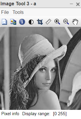
Output:

Explanation of code:

• MatLab program explanation for edge sharpening. a=imread(“cameraman.jpg”); This line reads the cameraman image in variable a.
• HBF=[0 -1 0; -1 5 -1; 0 -1 0]; This line defines the Laplacian filter.
• a1=conv2(a,HBF,’same’); This line convolves the image with HBF.
• After convolution, the values of some pixels go beyond the range [0 255]. Hence the next line is used.
• a2=uint8(a1); This line normalizes the pixel range.
• imtool(a2),[]) This line displays the sharpened image.
• SHBF=[-1 -1 -1; -1 8 -1; -1 -1 -1]; This line defines the strong HBF, with A=1 and Central=8
• a3=conv2(aSHBF,’ same’); This line convolves the original image with this filter.
• a4=uint8(a3); This line normalizes the range of pixel values.
• imtool(a4,[]) This line displays the sharpened image.