Image Segmentation using Python’s scikit-image module

The process of splitting images into multiple layers, represented by a smart, pixel-wise mask is known as Image Segmentation. It involves merging, blocking, and separating an image from its integration level. Splitting a picture into a collection of Image Objects with comparable properties is the first stage in image processing. Scikit-Image is the most popular tool/module for image processing in Python. 

Installation

To install this module type the below command in the terminal.

pip install scikit-image

Converting Image Format

RGB to Grayscale

rgb2gray module of skimage package is used to convert a 3-channel RGB Image to one channel monochrome image. In order to apply filters and other processing techniques, the expected input is a two-dimensional vector i.e. a monochrome image. 

skimage.color.rgb2gray() function is used to convert an RGB image to Grayscale format

Syntax : skimage.color.rgb2gray(image)

Parameters : image : An image – RGB format

Return : The image – Grayscale format

Code:

Python3

# Importing Necessary Libraries
from skimage import data
from skimage.color import rgb2gray
import matplotlib.pyplot as plt

# Setting the plot size to 15,15
plt.figure(figsize=(15, 15))

# Sample Image of scikit-image package
coffee = data.coffee()
plt.subplot(1, 2, 1)

# Displaying the sample image
plt.imshow(coffee)

# Converting RGB image to Monochrome
gray_coffee = rgb2gray(coffee)
plt.subplot(1, 2, 2)

# Displaying the sample image - Monochrome
# Format
plt.imshow(gray_coffee, cmap="gray")

Output:

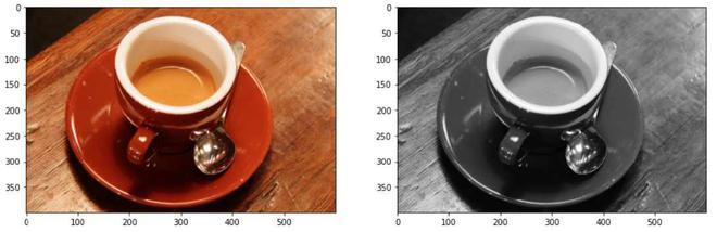
Converting 3-channel image data to 1-channel image data

Explanation: By using rgb2gray() function, the 3-channel RGB image of shape (400, 600, 3) is converted to a single-channel monochromatic image of shape (400, 300). We will be using grayscale images for the proper implementation of thresholding functions. The average of the red, green, and blue pixel values for each pixel to get the grayscale value is a simple approach to convert a color picture 3D array to a grayscale 2D array. This creates an acceptable gray approximation by combining the lightness or brightness contributions of each color band.

RGB to HSV

The HSV (Hue, Saturation, Value) color model remaps the RGB basic colors into dimensions that are simpler to comprehend for humans. The RGB color space describes the proportions of red, green, and blue in a colour. In the HSV color system, colors are defined in terms of Hue, Saturation, and Value.

skimage.color.rgb2hsv() function is used to convert an RGB image to HSV format

Syntax : skimage.color.rgb2hsv(image)

Parameters : image : An image – RGB format

Return : The image – HSV format

Code:

Python3

# Importing Necessary Libraries
from skimage import data
from skimage.color import rgb2hsv
import matplotlib.pyplot as plt

# Setting the plot size to 15,15
plt.figure(figsize=(15, 15))

# Sample Image of scikit-image package
coffee = data.coffee()
plt.subplot(1, 2, 1)

# Displaying the sample image
plt.imshow(coffee)

# Converting RGB Image to HSV Image
hsv_coffee = rgb2hsv(coffee)
plt.subplot(1, 2, 2)

# Displaying the sample image - HSV Format
hsv_coffee_colorbar = plt.imshow(hsv_coffee)

# Adjusting colorbar to fit the size of the image
plt.colorbar(hsv_coffee_colorbar, fraction=0.046, pad=0.04)

Output:

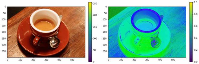
Converting the RGB color format to HSV color format

Supervised Segmentation

For this type of segmentation to proceed, it requires external input. This includes things like setting a threshold, converting formats, and correcting external biases.

Segmentation by Thresholding – Manual Input

An external pixel value ranging from 0 to 255 is used to separate the picture from the background. This results in a modified picture that is larger or less than the specified threshold.

Python3

# Importing Necessary Libraries
# Displaying the sample image - Monochrome Format
from skimage import data
from skimage import filters
from skimage.color import rgb2gray
import matplotlib.pyplot as plt

# Sample Image of scikit-image package
coffee = data.coffee()
gray_coffee = rgb2gray(coffee)

# Setting the plot size to 15,15
plt.figure(figsize=(15, 15))

for i in range(10):

  # Iterating different thresholds
  binarized_gray = (gray_coffee > i*0.1)*1
  plt.subplot(5,2,i+1)

  # Rounding of the threshold
  # value to 1 decimal point
  plt.title("Threshold: >"+str(round(i*0.1,1)))

  # Displaying the binarized image
  # of various thresholds
  plt.imshow(binarized_gray, cmap = 'gray')

plt.tight_layout()

Output:

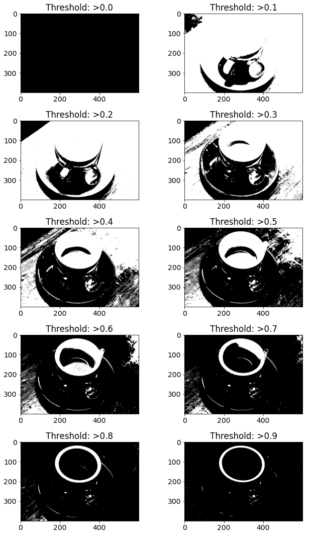
Explanation: The first step in this thresholding is implemented by normalizing an image from 0 – 255 to 0 – 1. A threshold value is fixed and on the comparison, if evaluated to be true, then we store the result as 1, otherwise 0. This globally binarized image can be used to detect edges as well as analyze contrast and color difference.

Segmentation by Thresholding  Using skimage.filters module

The Niblack and Sauvola thresholding technique is specifically developed to improve the quality of microscopic images. It’s a local thresholding approach that changes the threshold depending on the local mean and standard deviation for each pixel in a sliding window. Otsu’s thresholding technique works by iterating over all possible threshold values and computing a measure of dispersion for the sample points on either side of the threshold, i.e. either in foreground or background. The goal is to determine the smallest foreground and background spreads possible. 

skimage.filters.threshold_otsu() function is used to return threshold value based on Otsu’s method.

Syntax : skimage.filters.threshold_otsu(image)

Parameters :

• image : An image – Monochrome format
• nbins : Number of bins required for histogram calculation
• hist : Histogram from which threshold has to be calculated

Return : threshold : Larger pixel intensity 

skimage.filters.threshold_niblack() function is a local thresholding function that returns a threshold value for every pixel based on Niblack’s method.

Syntax : skimage.filters.threshold_niblack(image)

Parameters :

• image : An image – Monochrome format
• window_size : Window size – odd integer
• k : A positive parameter

Return : threshold : A threshold mask equal to the shape of the image

skimage.filters.threshold_sauvola() function is a local thresholding function that returns a threshold value for every pixel based on Sauvola’s method.

Syntax : skimage.filters.threshold_sauvola(image)

Parameters :

• image : An image – Monochrome format
• window_size : Window size – odd integer
• k : A positive parameter
• r : A positive parameter – dynamic range of standard deviation

Return : threshold : A threshold mask equal to the shape of the image

Code:

Python3

# Importing necessary libraries
from skimage import data
from skimage import filters
from skimage.color import rgb2gray
import matplotlib.pyplot as plt

# Setting plot size to 15, 15
plt.figure(figsize=(15, 15))

# Sample Image of scikit-image package
coffee = data.coffee()
gray_coffee = rgb2gray(coffee)

# Computing Otsu's thresholding value
threshold = filters.threshold_otsu(gray_coffee)

# Computing binarized values using the obtained
# threshold
binarized_coffee = (gray_coffee > threshold)*1
plt.subplot(2,2,1)
plt.title("Threshold: >"+str(threshold))

# Displaying the binarized image
plt.imshow(binarized_coffee, cmap = "gray")

# Computing Ni black's local pixel
# threshold values for every pixel
threshold = filters.threshold_niblack(gray_coffee)

# Computing binarized values using the obtained
# threshold
binarized_coffee = (gray_coffee > threshold)*1
plt.subplot(2,2,2)
plt.title("Niblack Thresholding")

# Displaying the binarized image
plt.imshow(binarized_coffee, cmap = "gray")

# Computing Sauvola's local pixel threshold
# values for every pixel - Not Binarized
threshold = filters.threshold_sauvola(gray_coffee)
plt.subplot(2,2,3)
plt.title("Sauvola Thresholding")

# Displaying the local threshold values
plt.imshow(threshold, cmap = "gray")

# Computing Sauvola's local pixel
# threshold values for every pixel - Binarized
binarized_coffee = (gray_coffee > threshold)*1
plt.subplot(2,2,4)
plt.title("Sauvola Thresholding - Converting to 0's and 1's")

# Displaying the binarized image
plt.imshow(binarized_coffee, cmap = "gray")

Output

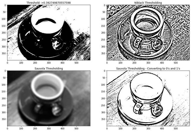
Explanation: These local thresholding techniques use mean and standard deviation as their primary computational parameters. Their final local pixel value is felicitated by other positive parameters too. This is done to ensure the separation between the object and the background. 

where \bar x and \sigma represents mean and standard deviation of the pixel intensities respectively.

Active Contour Segmentation

The concept of energy functional reduction underpins the active contour method. An active contour is a segmentation approach that uses energy forces and restrictions to separate the pixels of interest from the remainder of the picture for further processing and analysis. The term “active contour” refers to a model in the segmentation process. 

skimage.segmentation.active_contour() function active contours by fitting snakes to image features

Syntax : skimage.segmentation.active_contour(image, snake)

Parameters :

• image : An image
• snake : Initial snake coordinates – for bounding the feature
• alpha : Snake length shape
• beta : Snake smoothness shape
• w_line : Controls attraction – Brightness
• w_edge : Controls attraction – Edges
• gamma : Explicit time step

Return : snake : Optimised snake with input parameter’s size

Code:

Python3

# Importing necessary libraries
import numpy as np
import matplotlib.pyplot as plt
from skimage.color import rgb2gray
from skimage import data
from skimage.filters import gaussian
from skimage.segmentation import active_contour

# Sample Image of scikit-image package
astronaut = data.astronaut()
gray_astronaut = rgb2gray(astronaut)

# Applying Gaussian Filter to remove noise
gray_astronaut_noiseless = gaussian(gray_astronaut, 1)

# Localising the circle's center at 220, 110
x1 = 220 + 100*np.cos(np.linspace(0, 2*np.pi, 500))
x2 = 100 + 100*np.sin(np.linspace(0, 2*np.pi, 500))

# Generating a circle based on x1, x2
snake = np.array([x1, x2]).T

# Computing the Active Contour for the given image
astronaut_snake = active_contour(gray_astronaut_noiseless,
                                 snake)

fig = plt.figure(figsize=(10, 10))

# Adding subplots to display the markers
ax = fig.add_subplot(111)

# Plotting sample image
ax.imshow(gray_astronaut_noiseless)

# Plotting the face boundary marker
ax.plot(astronaut_snake[:, 0],
        astronaut_snake[:, 1],
        '-b', lw=5)

# Plotting the circle around face
ax.plot(snake[:, 0], snake[:, 1], '--r', lw=5)

Output:

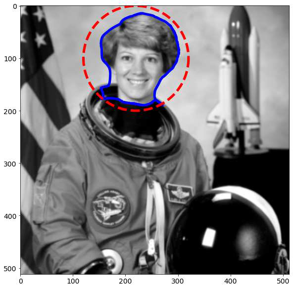
Explanation: The active contour model is among the dynamic approaches in image segmentation that uses the image’s energy restrictions and pressures to separate regions of interest. For segmentation, an active contour establishes a different border or curvature for each section of the target object. The active contour model is a technique for minimizing the energy function resulting from external and internal forces. An exterior force is specified as curves or surfaces, while an interior force is defined as picture data. The external force is a force that allows initial outlines to automatically transform into the forms of objects in pictures.

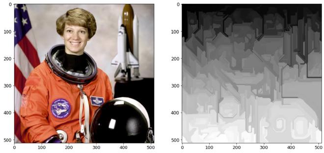
Chan-Vese Segmentation

The well-known Chan-Vese iterative segmentation method splits a picture into two groups with the lowest intra-class variance. This algorithm uses sets that are iteratively evolved to minimize energy, which is characterized by weights corresponding to the total of variations in intensity from the overall average outside the segmented region, the sum of differences from the overall average within the feature vector, and a term that is directly proportional to the length of the fragmented region’s edge.

skimage.segmentation.chan_vese() function is used to segment objects using the Chan-Vese Algorithm whose boundaries are not clearly defined.

Syntax : skimage.segmentation.chan_vese(image)

Parameters :

• image : An image
• mu : Weight – Edge Length
• lambda1 : Weight – Difference from average
• tol : Tolerance of Level set variation
• max_num_iter : Maximum number of iterations
• extended_output : Tuple of 3 values is returned

Return :

• segmentation : Segmented Image
• phi : Final level set
• energies: Shows the evolution of the energy

Code:

Python3

import matplotlib.pyplot as plt
from skimage.color import rgb2gray
from skimage import data, img_as_float
from skimage.segmentation import chan_vese
fig, axes = plt.subplots(1, 3, figsize=(10, 10))

# Sample Image of scikit-image package
astronaut = data.astronaut()
gray_astronaut = rgb2gray(astronaut)

# Computing the Chan VESE segmentation technique
chanvese_gray_astronaut = chan_vese(gray_astronaut,
                                    max_iter=100,
                                    extended_output=True)

ax = axes.flatten()

# Plotting the original image
ax[0].imshow(gray_astronaut, cmap="gray")
ax[0].set_title("Original Image")

# Plotting the segmented - 100 iterations image
ax[1].imshow(chanvese_gray_astronaut[0], cmap="gray")
title = "Chan-Vese segmentation - {} iterations".
format(len(chanvese_gray_astronaut[2]))

ax[1].set_title(title)

# Plotting the final level set
ax[2].imshow(chanvese_gray_astronaut[1], cmap="gray")
ax[2].set_title("Final Level Set")
plt.show()

Output:

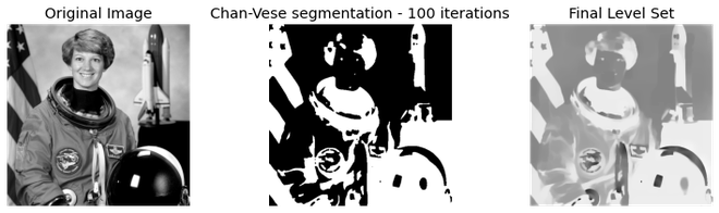
Explanation: The Chan-Vese model for active contours is a strong and versatile approach for segmenting a wide range of pictures, including some that would be difficult to segment using “traditional” methods such as thresholding or gradient-based methods. This model is commonly used in medical imaging, particularly for brain, heart, and trachea segmentation. The model is based on an energy minimization issue that may be recast in a level set formulation to make the problem easier to solve.

Unsupervised Segmentation

Mark Boundaries

This technique produces an image with highlighted borders between labeled areas, where the pictures were segmented using the SLIC method. 

skimage.segmentation.mark_boundaries() function is to return image with boundaries between labeled regions.

Syntax : skimage.segmentation.mark_boundaries(image)

Parameters :

• image : An image
• label_img : Label array with marked regions
• color : RGB color of boundaries
• outline_color : RGB color of surrounding boundaries

Return : marked : An image with boundaries are marked

Code:

Python3

# Importing required boundaries
from skimage.segmentation import slic, mark_boundaries
from skimage.data import astronaut

# Setting the plot figure as 15, 15
plt.figure(figsize=(15, 15))

# Sample Image of scikit-image package
astronaut = astronaut()

# Applying SLIC segmentation
# for the edges to be drawn over
astronaut_segments = slic(astronaut,
                          n_segments=100,
                          compactness=1)

plt.subplot(1, 2, 1)

# Plotting the original image
plt.imshow(astronaut)

# Detecting boundaries for labels
plt.subplot(1, 2, 2)

# Plotting the output of marked_boundaries
# function i.e. the image with segmented boundaries
plt.imshow(mark_boundaries(astronaut, astronaut_segments))

Output:

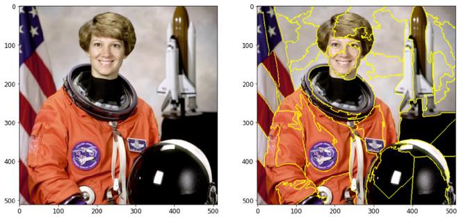
Explanation: We cluster the image into 100 segments with compactness = 1 and this segmented image will act as a labeled array for the mark_boundaries() function. Each segment of the clustered image is differentiated by an integer value and the result of mark_boundaries is the superimposed boundaries between the labels.

Simple Linear Iterative Clustering

By combining pixels in the image plane based on their color similarity and proximity, this method generates superpixels. Simple Linear Iterative Clustering is the most up-to-date approach for segmenting superpixels, and it takes very little computing power. In a nutshell, the technique clusters pixels in a five-dimensional color and picture plane space to create small, nearly uniform superpixels.

skimage.segmentation.slic() function is used to segment image using k-means clustering.

Syntax : skimage.segmentation.slic(image)

Parameters :

• image : An image
• n_segments : Number of labels
• compactness : Balances color and space proximity.
• max_num_iter : Maximum number of iterations

Return : labels: Integer mask indicating segment labels.

Code:

Python3

# Importing required libraries
from skimage.segmentation import slic
from skimage.data import astronaut
from skimage.color import label2rgb

# Setting the plot size as 15, 15
plt.figure(figsize=(15,15))

# Sample Image of scikit-image package
astronaut = astronaut()

# Applying Simple Linear Iterative
# Clustering on the image
# - 50 segments & compactness = 10
astronaut_segments = slic(astronaut,
                          n_segments=50,
                          compactness=10)
plt.subplot(1,2,1)

# Plotting the original image
plt.imshow(astronaut)
plt.subplot(1,2,2)

# Converts a label image into
# an RGB color image for visualizing
# the labeled regions.
plt.imshow(label2rgb(astronaut_segments,
                     astronaut,
                     kind = 'avg'))

Output:

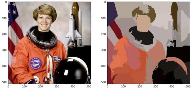
Explanation: This technique creates superpixels by grouping pixels in the picture plane based on their color similarity and closeness. This is done in 5-D space, where XY is the pixel location. Because the greatest possible distance between two colors in CIELAB space is restricted, but the spatial distance on the XY plane is dependent on the picture size, we must normalize the spatial distances in order to apply the Euclidean distance in this 5D space. As a result, a new distance measure that takes superpixel size into account was created to cluster pixels in this 5D space. 

Felzenszwalb’s Segmentation

Felsenszwalb’s efficient graph-based picture segmentation is computed. It produces an over-segmentation of an RGB picture on the image grid using a quick, minimal spanning tree-based clustering. This may be used to isolate features and identify edges. This algorithm uses the Euclidean distance between pixels. skimage.segmentation.felzenszwalb() function is used to compute Felsenszwalb’s efficient graph-based image segmentation.  

Syntax : skimage.segmentation.felzenszwalb(image)

Parameters :

• image : An input image
• scale : Higher value – larger clusters
• sigma : Width of Gaussian kernel
• min_size : Minimum component size

Return : segment_mask : Integer mask indicating segment labels. 

Code:

Python3

# Importing the required libraries
from skimage.segmentation import felzenszwalb
from skimage.color import label2rgb
from skimage.data import astronaut

# Setting the figure size as 15, 15
plt.figure(figsize=(15,15))

# Sample Image of scikit-image package
astronaut = astronaut()

# computing the Felzenszwalb's
# Segmentation with sigma = 5 and minimum
# size = 100
astronaut_segments = felzenszwalb(astronaut,
                                  scale = 2,
                                  sigma=5,
                                  min_size=100)

# Plotting the original image
plt.subplot(1,2,1)
plt.imshow(astronaut)

# Marking the boundaries of
# Felzenszwalb's segmentations
plt.subplot(1,2,2)
plt.imshow(mark_boundaries(astronaut,
                           astronaut_segments))

Output:

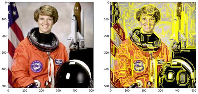
With mark_boundaries() function

Without mark_boundaries() function

Explanation: Using a rapid, minimal tree structure-based clustering on the picture grid, creates an over-segmentation of a multichannel image. The parameter scale determines the level of observation. Less and larger parts are associated with a greater scale. The diameter of a Gaussian kernel is sigma, which is used to smooth the picture before segmentation. Scale is the sole way to control the quantity of generated segments as well as their size. The size of individual segments within a picture might change dramatically depending on local contrast.

There are many other supervised and unsupervised image segmentation techniques. This can be useful in confining individual features, foreground isolation, noise reduction, and can be useful to analyze an image more intuitively. It is a good practice for images to be segmented before building a neural network model in order to yield effective results.