IBM HR Analytics on Employee Attrition & Performance using Random Forest Classifier

Attrition is a problem that impacts all businesses, irrespective of geography, industry and size of the company. It is a major problem to an organization, and predicting turnover is at the forefront of the needs of Human Resources (HR) in many organizations. Organizations face huge costs resulting from employee turnover. With advances in machine learning and data science, it’s possible to predict the employee attrition, and we will predict using Random Forest Classifier algorithm. 

Dataset: The dataset that is published by the Human Resource department of IBM is made available at Kaggle.

Code: Implementation of Random Forest Classifier algorithm for classification.

Code: Loading the Libraries

Python3

# performing linear algebra
import numpy as np

# data processing
import pandas as pd

# visualisation
import matplotlib.pyplot as plt
import seaborn as sns % matplotlib inline

Code: Importing the dataset

Python3

dataset = pd.read_csv("WA_Fn-UseC_-HR-Employee-Attrition.csv")
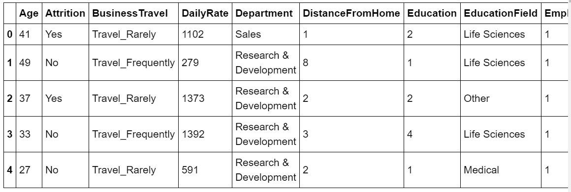
print (dataset.head)

Output :

Code: Information about the dataset

Python3

dataset.info()

Output :

RangeIndex: 1470 entries, 0 to 1469
Data columns (total 35 columns):
Age                         1470 non-null int64
Attrition                   1470 non-null object
BusinessTravel              1470 non-null object
DailyRate                   1470 non-null int64
Department                  1470 non-null object
DistanceFromHome            1470 non-null int64
Education                   1470 non-null int64
EducationField              1470 non-null object
EmployeeCount               1470 non-null int64
EmployeeNumber              1470 non-null int64
EnvironmentSatisfaction     1470 non-null int64
Gender                      1470 non-null object
HourlyRate                  1470 non-null int64
JobInvolvement              1470 non-null int64
JobLevel                    1470 non-null int64
JobRole                     1470 non-null object
JobSatisfaction             1470 non-null int64
MaritalStatus               1470 non-null object
MonthlyIncome               1470 non-null int64
MonthlyRate                 1470 non-null int64
NumCompaniesWorked          1470 non-null int64
Over18                      1470 non-null object
OverTime                    1470 non-null object
PercentSalaryHike           1470 non-null int64
PerformanceRating           1470 non-null int64
RelationshipSatisfaction    1470 non-null int64
StandardHours               1470 non-null int64
StockOptionLevel            1470 non-null int64
TotalWorkingYears           1470 non-null int64
TrainingTimesLastYear       1470 non-null int64
WorkLifeBalance             1470 non-null int64
YearsAtCompany              1470 non-null int64
YearsInCurrentRole          1470 non-null int64
YearsSinceLastPromotion     1470 non-null int64
YearsWithCurrManager        1470 non-null int64
dtypes: int64(26), object(9)
memory usage: 402.0+ KB

Code: Visualizing the data

Python3

# heatmap to check the missing value
plt.figure(figsize =(10, 4))
sns.heatmap(dataset.isnull(),
            yticklabels = False,
            cbar = False,
            cmap ='viridis')

Output:

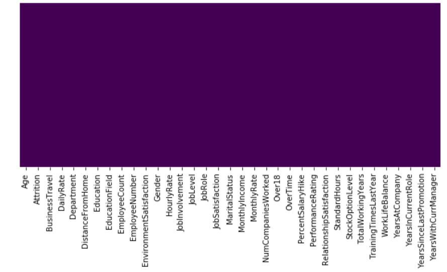
So, we can see that there are no missing values in the dataset. This is a Binary Classification Problem, so the Distribution of instances among the 2 classes, is visualized below :

Code:

Python3

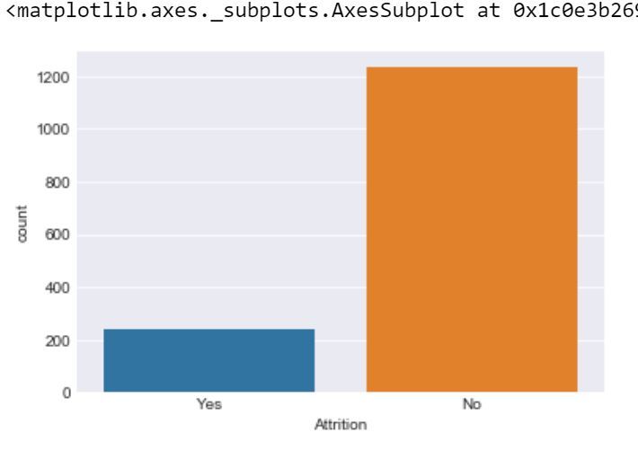
sns.set_style('darkgrid')
sns.countplot(x ='Attrition',
              data = dataset)

Output:

Code:

Python3

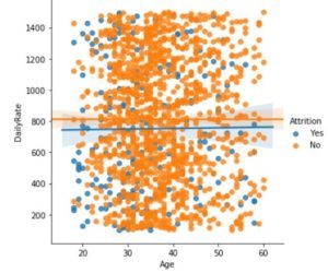
sns.lmplot(x = 'Age',
           y = 'DailyRate',
           hue = 'Attrition',
           data = dataset)

Output:

Code:

Python3

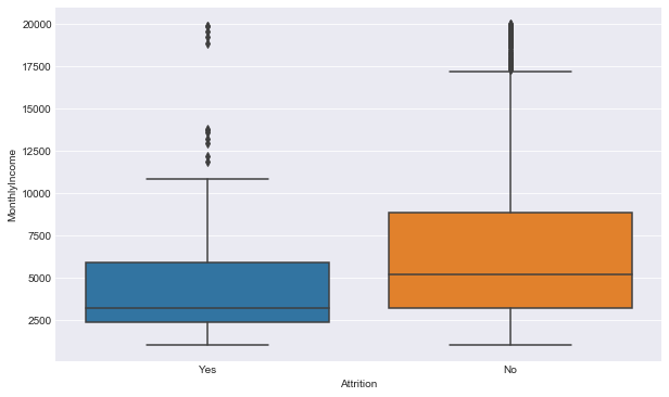
plt.figure(figsize =(10, 6))
sns.boxplot(y ='MonthlyIncome',
            x ='Attrition',
            data = dataset)

Output:

Code: Preprocessing the data

In the dataset there are 4 irrelevant columns, i.e:EmployeeCount, EmployeeNumber, Over18, and StandardHour. So, we have to remove these for more accuracy.

Python3

dataset.drop('EmployeeCount',
             axis = 1,
             inplace = True)
dataset.drop('StandardHours',
             axis = 1,
             inplace = True)
dataset.drop('EmployeeNumber',
             axis = 1,
             inplace = True)
dataset.drop('Over18',
             axis = 1,
             inplace = True)

print(dataset.shape)

Output:

(1470, 31)

So, we have removed the irrelevant column.

Code: Input and Output data

Python3

y = dataset.iloc[:, 1]
X = dataset

X.drop('Attrition',
       axis = 1,
       inplace = True)

Code: Label Encoding

Python3

from sklearn.preprocessing import LabelEncoder
lb = LabelEncoder()
y = lb.fit_transform(y)

In the dataset there are 7 categorical data, so we have to change them to int data, i.e we have to create 7 dummy variables for better accuracy.

Code: Dummy variable creation

Python3

dum_BusinessTravel = pd.get_dummies(dataset['BusinessTravel'],
                                    prefix ='BusinessTravel')

dum_Department = pd.get_dummies(dataset['Department'],
                                prefix ='Department')

dum_EducationField = pd.get_dummies(dataset['EducationField'],
                                   prefix ='EducationField')

dum_Gender = pd.get_dummies(dataset['Gender'],
                           prefix ='Gender', drop_first = True)

dum_JobRole = pd.get_dummies(dataset['JobRole'],

                            prefix ='JobRole')

dum_MaritalStatus = pd.get_dummies(dataset['MaritalStatus'],

                                  prefix ='MaritalStatus')

dum_OverTime = pd.get_dummies(dataset['OverTime'],
                             prefix ='OverTime', drop_first = True)

# Adding these dummy variable to input X
X = pd.concat([x, dum_BusinessTravel, dum_Department,
              dum_EducationField, dum_Gender, dum_JobRole,
              dum_MaritalStatus, dum_OverTime], axis = 1)

# Removing the categorical data
X.drop(['BusinessTravel', 'Department', 'EducationField',
       'Gender', 'JobRole', 'MaritalStatus', 'OverTime'],
       axis = 1, inplace = True)

print(X.shape)
print(y.shape)

Output:

(1470, 49)
(1470, )

Code: Splitting data to training and testing

Python3

from sklearn.model_selection import train_test_split

X_train, X_test, y_train, y_test = train_test_split(

   X, y, test_size = 0.25, random_state = 40)

So, the preprocessing is done, now we have to apply the Random forest classifier to the dataset. 

Code: Model Execution

Python3

from sklearn.model_selection import cross_val_predict, cross_val_score
from sklearn.metrics import accuracy_score, classification_report, confusion_matrix
from sklearn.ensemble import RandomForestClassifier

rf = RandomForestClassifier(n_estimators=10,
                            criterion='entropy')
rf.fit(X_train, y_train)
y_pred = rf.predict(X_test)

def print_score(clf, X_train, y_train,
                X_test, y_test,
                train=True):

    if train:
        print("Train Result:")
        print("------------")
        print("Classification Report: \n {}\n".format(classification_report(
            y_train, clf.predict(X_train))))

        print("Confusion Matrix: \n {}\n".format(confusion_matrix(
            y_train, clf.predict(X_train))))

        res = cross_val_score(clf, X_train, y_train,
                              cv=10, scoring='accuracy')

        print("Average Accuracy: \t {0:.4f}".format(np.mean(res)))
        print("Accuracy SD: \t\t {0:.4f}".format(np.std(res)))
        print("----------------------------------------------------------")

    elif train == False:

        print("Test Result:")
        print("-----------")
        print("Classification Report: \n {}\n".format(
            classification_report(y_test, clf.predict(X_test))))

        print("Confusion Matrix: \n {}\n".format(
            confusion_matrix(y_test, clf.predict(X_test))))

        print("accuracy score: {0:.4f}\n".format(
            accuracy_score(y_test, clf.predict(X_test))))

        print("-----------------------------------------------------------")

print_score(rf, X_train, y_train,
            X_test, y_test,
            train=True)

print_score(rf, X_train, y_train,
            X_test, y_test,
            train=False)

Output:

Train Result:
------------
Classification Report: 
               precision    recall  f1-score   support

           0       0.98      1.00      0.99       988
           1       1.00      0.90      0.95       188

    accuracy                           0.98      1176
   macro avg       0.99      0.95      0.97      1176
weighted avg       0.98      0.98      0.98      1176


Confusion Matrix: 
 [[988   0]
 [ 19 169]]

Average Accuracy:      0.8520
Accuracy SD:          0.0122
----------------------------------------------------------
Test Result:
-----------
Classification Report: 
               precision    recall  f1-score   support

           0       0.86      0.98      0.92       245
           1       0.71      0.20      0.32        49

    accuracy                           0.85       294
   macro avg       0.79      0.59      0.62       294
weighted avg       0.84      0.85      0.82       294


Confusion Matrix: 
 [[241   4]
 [ 39  10]]

accuracy score: 0.8537

-----------------------------------------------------------

Code: Key features for deciding the result

Python3

pd.Series(rf.feature_importances_,
         index = X.columns).sort_values(ascending = False).plot(kind = 'bar',
                                                                figsize = (14,6));

Output:

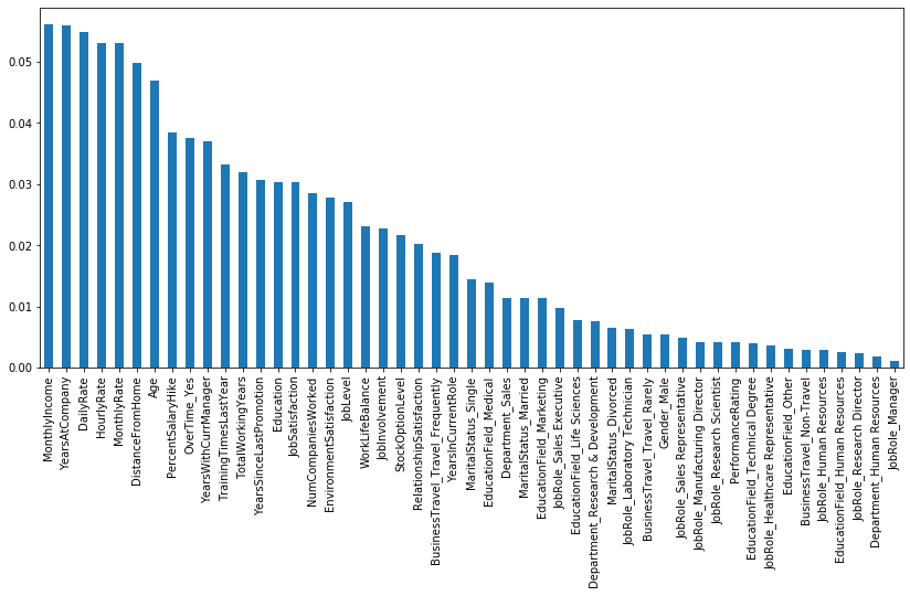
So, According to Random forest classifier the most important feature for predicting the result is Monthly Income and the least important feature is jobRole_Manager.