How to Sum Values Based on Criteria in Another Column in Excel?

In Excel, we can approach the problem in two ways. [SUMIF Formula and Excel Pivot]

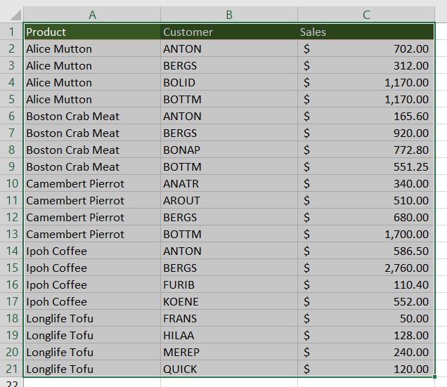
Sample data: Sales Report Template

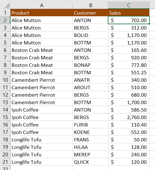
We are creating a summary table for Total Product sales.  

Approach 1: Excel Formula SUMIF

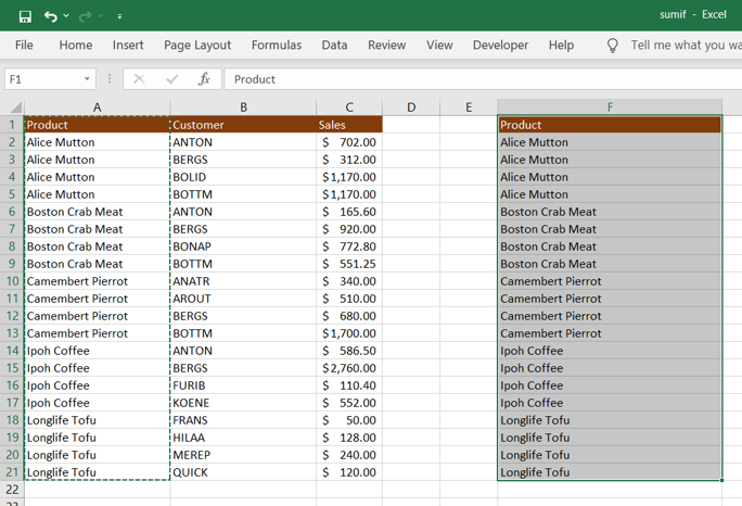
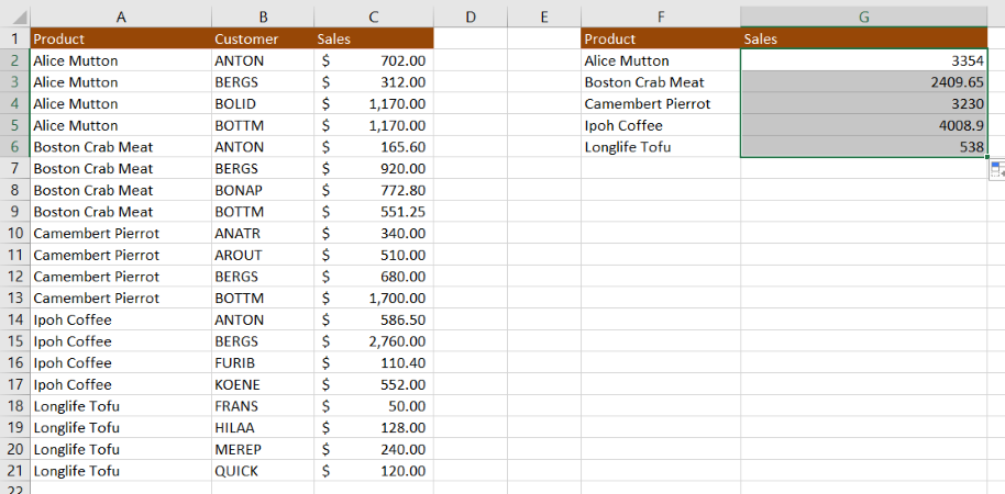
Step 1: Copy “Column A” Products and then paste into “Column F”

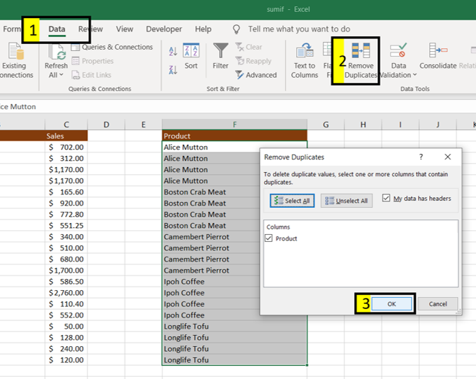
Step 2: Remove duplicate products in “Column F”

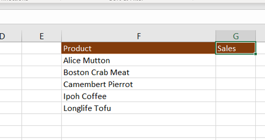
Step 3: Type “Sales” in cell G1.

Step 4: Now make use of the below formula.

Syntax:

SUMIF(range, criteria, [sum_range])

Where,

• range : Required. Excel range of cells, to apply criteria.
• criteria : Required.  criteria example : 12, “>12”, t7, “5?” or “blue*”.
• sum_range : optional.  Excel range to add 

Now write SUMIF() in cell G2

=SUMIF($A$1:$A$21,F2,$C$1:$C$21) 

Step 5: Select cell G2 and drag till cell G6

Approach 2: Using Pivot table

Step 1: Select the entire data range (A1:C21)

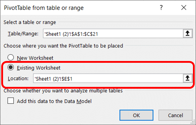
Step 2: Now click Insert >> PivotTable to open the Create PivotTable dialog box

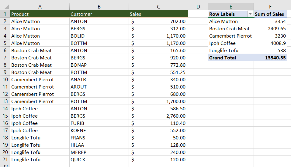
Step 3: In the PivotTable Fields pane, drag the criteria column name (Product) to the Rows section, drag the column you will sum (Sales), and move to the Values section

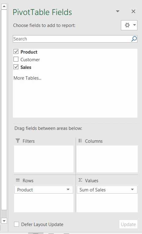
Pivot Table: Total Products Sales [Column E and F]

My Personal Notes arrow_drop_up

Save