How to Sum Diagonal Cells in a range in Excel?

The calculation of matrices is one of the most difficult numerical computation tasks. You may need to add values diagonally in a table when performing mathematical computations. Excel allows you to sum diagonal numbers without having to add the values one by one.  We’ll go through how to sum cells diagonally down or diagonally up.

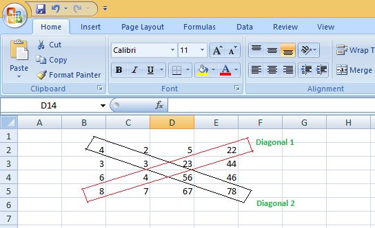
Example: The image below shows a matrix & we want to add the elements of the diagonal. Diagonal1 is the right diagonal & Diagonal2 is the left diagonal as its top element is on the left.

Conditional Formatting (On Matrix or Table) :

To do conditional formatting use the following steps :
Step 1: Select the Matrix/Table. Then Go to the home tab & select the conditional formatting option.

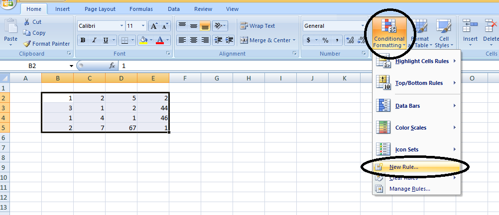
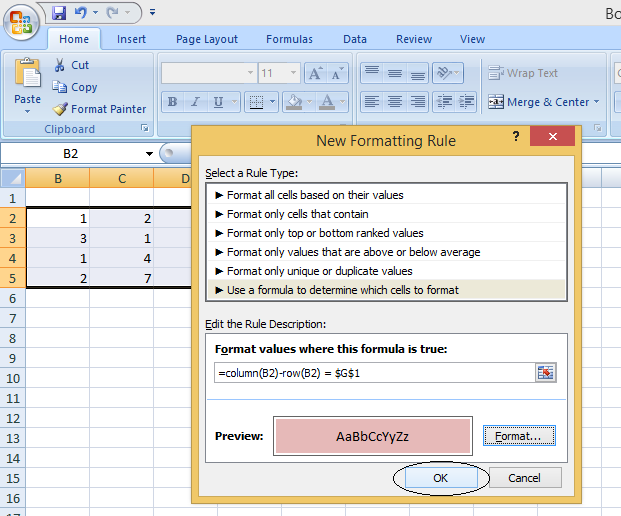
Step 2: Choose New Rule.

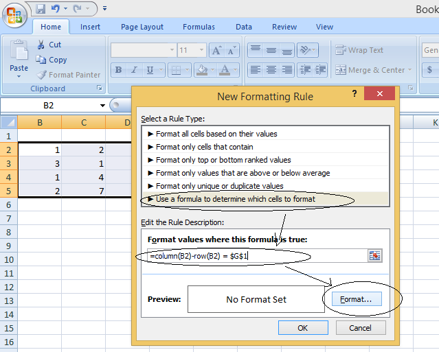
Step 3: Select: “Use a formula to determine which cells to format” & in the rule description give the format values for the formula. Here we give 1st cell name of the matrix in the formula, i.e., column(B2) – row(B2) (For diagonal)

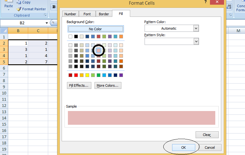
Step 4: Click on the format. Choose the color, fonts, etc, for formatting & then click on OK.

Step 6: Click on Ok.

You will get your cells formatted.

How to Sum Diagonal Cells in a range in Excel?

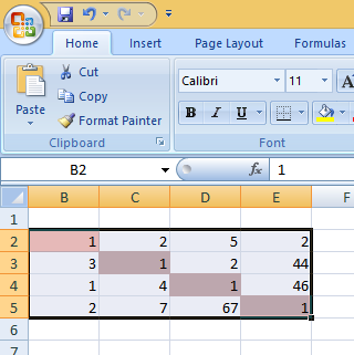
A range of cells containing values can be seen in the image below :

Steps to sum the elements diagonally down(from top to bottom) :

Check the cell ranges, say, ‘B2’ is the first upper-left cell. This is significant because cell ‘B2’ serves as the start point for the diagonal sum. We SUM the diagonal values down from the first cell ‘B2’ diagonally right till ‘E5’.

Here we want right the diagonal sum, i.e., sum of the cells: B2+C3+D4+E5 . 
To do sum of the Left diagonal  we will use the formula :

=SUM((COLUMN(Cells Reference)-ROW(Cells Reference) =cellName )*Cells Reference) 
into a blank cell , Say F6

Step 1: Go to the cell, where you want to get the result of the addition.

Step 2 : There write : =SUM((COLUMN(B2:E5)-ROW(B2:E5)=M1)*B2:E5)

Step 3 : Press Ctrl + Shift + Enter.

You will get the left diagonal sum. Here you can see the left diagonal sum = 1+1+1+1 = 4

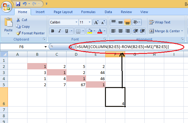
Note: Here M1 contains the difference between columns & rows. Currently, in the above image, it is 0.

If we go to M1 & change its value to 2 :

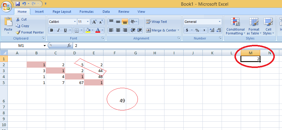
The addition now is changed to 49 which is the sum of D2 + E3 , i.e., 44+5 = 9. The value 2 of M here indicates the diagonal 2 steps above the current diagonal(in other way we exclude 2 columns & 2 rows)

If we go to M1 & change its value to -1 :

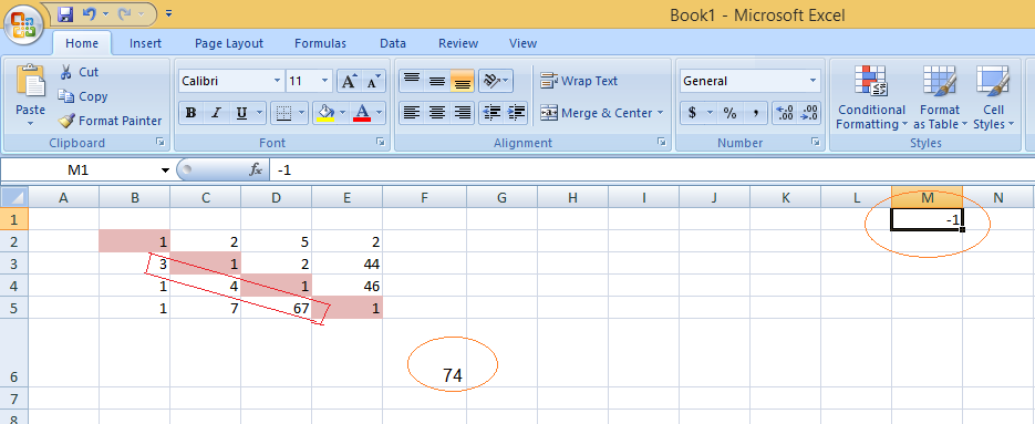
The addition now is changed to 74 which is the sum of B3 + C4 + D5 , i.e., 3+4+67. The value -1 of M here indicates the diagonal 1 step below the current diagonal(in other way we exclude 1 column & 1 row downwards)

Steps to sum the elements diagonally up(from bottom) / The SUM of Diagonal Cells Ascending from Left to Right :

Check the cell ranges, say, ‘E2’ is the first upper right cell. This is significant because cell ‘B5’ serves as the start point for the diagonal sum. We SUM the diagonal values down from the first cell ‘E2’ diagonally right till ‘B5’.

Here we want right the diagonal sum , i.e., sum of the cells: E2+D3+C4+B5. To do sum of the right diagonal  we will use the formula :

=SUM(Cell Reference*((ROWS(Cell Reference) + Ri)-ROW(Cell Reference)=COLUMN(Cell Reference)-Ci)) 
into a blank cell , Say F6
Ri => the number of rows in front of the data range's initial cell.
Ci => the number of columns in front of the data range's initial cell.

Example 1: If you have a 5*5 matrix from Row 1 & column A (i.e., From A1 to E5), then if we formula :

= SUM(A1:E5*((ROWS(A1:E5)+0)-ROW(A1:E5)=COLUMN(A1:E5)))

Here Ri = 0, then the no of rows in front of the first cell of the data range is 0, so the addition is done for:  A4+ B3 + C2 + D1

Example 2 :

Step 1: Go to the cell, where you want to get the result of the addition.

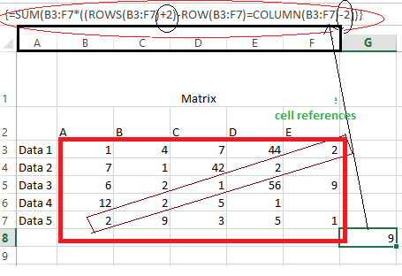
Step 2 : There write : =SUM(B2:E5*((ROWS(B2:E5)+2)-ROW(B2:E5)=COLUMN(B2:E5)-1))

Step 3 : Press Ctrl + Shift + Enter.

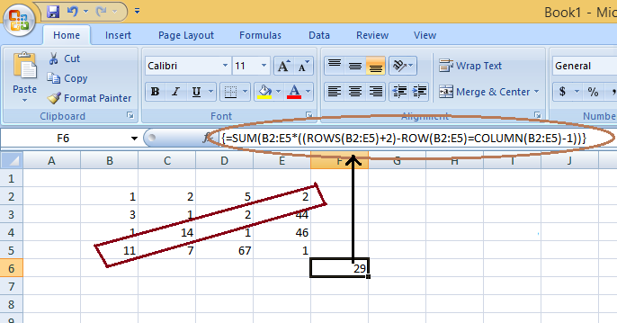
You will get the left diagonal sum. Here you can see the right diagonal sum = 11+14+2+2 = 29

The Diagonal Sum of Values in an Excel table if the number of columns and rows is the same :

In the above example also we have the same number of rows & columns in the cell range. But the thing in the below example differ is that there are different numbers of columns & rows in front of the cell range.

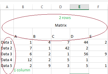
Suppose we want to calculate sum of the elements diagonally up :

Here, C_i = 2 & R_i  = 2: as the number of rows in front of the cell reference is 2 & the number of columns in front of the actual cell references is 1.

The Diagonal Sum of Values in the Excel table if the number of columns and rows is different :

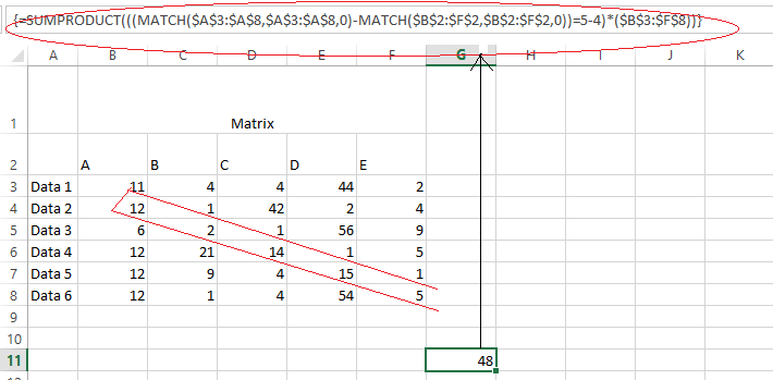
In the image below, you can see that the number of rows = 6 & the number of columns = 5 in the cell references.
To find the diagonal sum, follow these steps :

Step 1: Go to the cell, where you want to get the result of the addition.

Step 2: There write : = SUMPRODUCT(((MATCH($A$3:$A$8,$A$3:$A$8,0)-MATCH($B$2:$F$2,$B$2:$F$2,0))=5-4)*($B$3:$F$8))

Step 3: Press Ctrl + Shift + Enter.

Sum of Diagonal Values per column :

The basic formula comes next if we wish to start at the beginning and multiply the total of the numbers or values diagonally by the start column of cell ‘B3’. Take note of the number of rows labeled ‘pink’  in the calculation below.

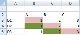
= SUMPRODUCT(((MATCH($A$3:$A$5,$A$3:$A$5,0)-MATCH($B$2:$D$2,$B$2:$D$2,0))=1-1)*($B$3:$D$5))
= SUMPRODUCT((((ROW($A$3:$A$5)-1)-(COLUMN($B$2:$D$2)-2))=3-1)*($B$3:$D$5))

The Diagonal Sum Down for a specific Number of Columns :

Use the ARRAY formula below to get the sum of the values diagonally down for a certain number of columns. The formula is found in cell ‘I11’ in the image above, while the condition ‘number 3’ is found in cell ‘G11’ in the image above. Only the first 4 columns of the data range are included in this calculation, which is the diagonal sum of values (enter the formula in one line).

= SUM(IF(ROW(OFFSET($B$3:$F$8,0,0,$G$11,G11))-MAX(ROW(OFFSET($B$3:$F$8,0,0,$G$11,G11)))=
COLUMN(OFFSET($B$3:$F$8,0,0,$G$11,G11))-MAX(COLUMN(OFFSET($B$3:$F$8,0,0,$G$11,G11))),
OFFSET($B$3:$F$8,0,0,$G$11,G11),FALSE))

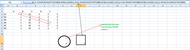
Note that here, in G11, we are specifying the column up to which we want to sum the diagonal elements.