How to Solve Histogram Equalization Numerical Problem in MATLAB?

Difficulty Level : Expert
Last Updated : 22 Nov, 2021

Histogram Equalization is a mathematical technique to widen the dynamic range of the histogram. Sometimes the histogram is spanned over a short range, by equalization the span of the histogram is widened. In digital image processing, the contrast of an image is enhanced using this very technique.

Use of Histogram Equalization:

It is used to increase the spread of the histogram. If the histogram represents the digital image, then by spreading the intensity values over a large dynamic range we can improve the contrast of the image.

Algorithm:

Find the frequency of each value represented on the horizontal axis of the histogram i.e. intensity in the case of an image.
Calculate the probability density function for each intensity value.
After finding the PDF, calculate the cumulative density function for each intensity’s frequency.
The CDF value is in the range 0-1, so we multiply all CDF values by the largest value of intensity i.e. 255.
Round off the final values to integer values.

Example:

Matlab

% MATLAB code for Histogram equalisation
% function to return resultant
% matrix and summary
function [f,r]=HistEq(k,max)
Freq=zeros(1,max);
[x,y]=size(k);
  
% Calculate frequency of each
% intensity value.
for i=1:x
    for j=1:y
        Freq(k(i,j)+1)=Freq(k(i,j)+1)+1;
    end
end
  
% Calculate PDF for each intensity value.
PDF=zeros(1,max);
Total=x*y;
for i=1:max
    PDF(i)=Freq(i)/Total;
end
  
% Calculate the CDF for each intensity value.
CDF=zeros(1,max);
CDF(1)=PDF(1);
for i=2:max
    CDF(i)=CDF(i-1)+PDF(i);
end
  
% Multiply by Maximum intensity value
% and round off the result.
Result=zeros(1,max);
for i=1:max
    Result(i)=uint8(CDF(i)*(max-1));
end
  
% Compute the Equalized image/matrix.
mat=zeros(size(k));
for i=1:x
    for j=1:y
        mat(i,j)=Result(k(i,j)+1);
    end
end
    
f=mat;
r=Result;
end
  
% Utility code here.
k=[0, 1, 1, 3, 4; 
   7, 2, 5, 5, 7; 
   6, 3, 2, 1, 1; 
   1, 4, 4, 2, 1];
     
[new_matrix, summary]=HistEq(k,8);

Output:

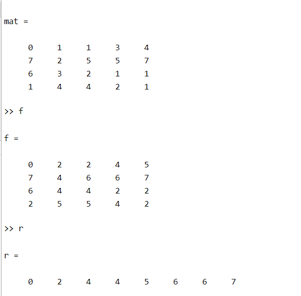
A 3-bit image of size 4×5 is shown below. Compute the histogram equalized image.

0	1	1	3	4
7	2	5	5	7
6	3	2	1	1
1	4	4	2	1

Steps:

Find the range of intensity values.
Find the frequency of each intensity value.
Calculate the probability density function for each frequency.
Calculate the cumulative density function for each frequency.
Multiply CDF with the highest intensity value possible.
Round off the values obtained in step-5.

Overview of calculation:
Range of intensity values = [0, 1, 2, 3, 4, 5, 6, 7]
Frequency of values = [1,  6, 3, 2, 3, 2, 1, 2] 
total = 20 = 4*5
Calculate PDF = frequency of each intensity/Total sum of
all frequencies, for each i value of intensity
Calculate CDF =cumulative frequency of each intensity 
value = sum of all PDF value (<=i)
Multiply CDF with 7.
Round off the final value of intensity.

The tabular form of the calculation is given here:

Range	Frequency	PDF	CDF	*7CDF**	Round-off
0	1	0.0500	0.0500	0.3500	0
1	6	0.3000	0.3500	2.4500	2
2	3	0.1500	0.5000	3.5000	4
3	2	0.1000	0.6000	4.2000	4
4	3	0.1500	0.7500	5.2500	5
5	2	0.1000	0.8500	5.9500	6
6	1	0.0500	0.9000	6.3000	6
7	2	0.1000	1.0000	7.0000	7

Interpretation: 
The pixel intensity in the image has modified.
0 intensity is replaced by 0.
1 intensity is replaced by 2.
2 intensity is replaced by 4.
3 intensity is replaced by 4.
4 intensity is replaced by 5.
5 intensity is replaced by 6.
6 intensity is replaced by 6.
7 intensity is replaced by 7.

Output: The new image is as follow:

0	2	2	4	5
7	4	6	6	7
6	4	4	2	2
2	5	5	4	2

My Personal Notes

Related Articles

Table of Contents

How to Solve Histogram Equalization Numerical Problem in MATLAB?

Use of Histogram Equalization:

Algorithm:

Matlab

Start Your Coding Journey Now!