How to make a 3 Axis Graph using Excel?

3 Axis Graphs in Excel are the graphs that have three axis. The need for a three-axis arises when the scale of the values is very different. For example, you are given an atom and you want to make a graph between its diameter, melting point, and colloidal nature. If they are plotted on the same scale then the diameter values will be represented as a single line as the melting point will be very value than its diameter. To resolve, this problem you need to have 3 axis for plotting all three different scale values. In this article, we will learn how to create a three-axis graph in excel. 

Creating a 3 axis graph

By default, excel can make at most two axis in the graph. There is no way to make a three-axis graph in excel. The three axis graph which we will make is by generating a fake third axis from another graph. Given a data set, of date and corresponding three values Temperature, Pressure, and Volume. Make a three-axis graph in excel. 

To create a 3 axis graph follow the following steps:

Step 1: Select table B3:E12. Then go to Insert Tab, and select the Scatter with Chart Lines and Marker Chart. 

Step 2: A Line chart with a primary axis will be created.  

Step 3: The primary axis of the chart will be Temperature, the secondary axis will be Pressure and the third axis will be Volume. So, to create the third axis duplicate this chart by pressing Ctrl + D while selecting graph1. Let’s name chart1 as graph1 and chart2 as graph2.Graph1 will contain the Primary and the secondary axis. The third axis will be created by graph2.

Step 4: As graph1 contains Volume which will be the third axis, you need to delete Volume from graph1. Double click on the red line and press Delete.  

Step 5: You have to make Pressure as the secondary axis in graph1. Double click, on the blue line. A Format Data Series dialogue box appears. In the series Option, select the blue line as the Secondary Axis. 

Step 6: Now, you need to remove the Chart Title of graph1. Double click on the chart title of graph1. Format Chart Title dialogue box appears. Go to Text options. In the Text Fill, select No Fill.

Step 7: You need to make graph1 transparent and with no border so that the overlapping could be done efficiently. Double click on the chart area of graph1. Format Chart Area dialogue box appears. In Chart Options, under the Fill section select No fill, and under the Border section select No line. The design of graph1 is over now. 

Step 8: Now, you need to remove all the gridlines of the entire worksheet. Go to View Tab, and uncheck the box Gridlines. 

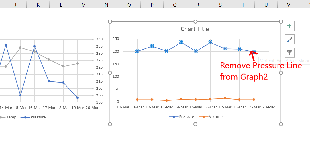
Step 9: You need to repeat the same steps with graph2 also. In graph2, we need only the third axis i.e. Volume. So, we will remove the rest of the two lines from graph2. Double click on the Temp line and press Delete. Again, double-click on the Pressure line and press Delete. 

Step 10: You, need to remove the Chart title from graph2 also. Double click on the Chart title in graph2. 

Step 11: Format Chart Title dialogue box appears. In the Text Options, under Text Fill select No Fill. 

Step 12: You need to make graph2 transparent and with no border so that the overlapping could be done efficiently. Double click on the chart area of graph2. Format Chart Area dialogue box appears. In Chart Options, under the Fill section select No fill, and under the Border section select No line. The design of graph2 is over now.

Step 13: Both graphs look like this now. 

Step 14: You need to add an axis title to every axis. Select graph1, and click on the plus button. Check the box, Axis Titles. 

Step 15: Axis title will appear in both the axis of graph1. 

Step 16: Now, you have to edit and design the data labels and axis titles on each axis. Double click, the Axis title on the secondary axis. Rename it to Pressure, color to blue, and size as per your comfortability. 

Step 17: Double click on the data labels in graph1. Set color to blue and size accordingly. 

Step 18: Again, double click on the data label of the secondary axis in graph1. Format Axis dialogue box appears. In Axis Options, under Line sections select the color of the axis line and its width. For example, color to blue and width to 2.5pt. 

Step 19: Repeat steps 16, 17, and 18 to design the primary axis of graph1. Set color to grey and width accordingly. 

Step 20: We see a problem that tick marks are not appearing in the primary axis of graph1. 

Step 21: Double click on the data label of the primary axis of graph1. Format Axis dialogue box appears. In Axis Options, under Tick Marks, select Major Type as Outside.  

Step 22: Repeat steps 16, 17, and 18 to design the primary axis of graph2. Set color to red and width accordingly.

Step 23: Both the graphs are ready. Now, you need to remove the dates from one of the graphs, so that they do not overlap. Removing the dates of graph2. 

Step 24: We know that dates can be represented in number format in excel. We see that the largest date in the given data set is 19-Mar whose number represented in excel is 44639. The dates value of graph2 are to be set such that they align with the dates of graph1, this could be achieved by the hit and trial method, checking the different maximum and minimum values, and seeing the best-suited value. Double click on the date in graph2. Format Axis dialogue box appears. In the Axis options, change the minimum from 44630 to 44628 and the maximum from 44640 to 44639. 

Step 25: By decreasing the minimum value, a space will be created between the data line and the start of the graph, this is necessary to avoid overlapping when placing graph2 over graph1. The maximum value is set as the largest date in the given data set, for example, 19-march in this case, this is necessary so that the graph lines of graph1 are aligned with the graph lines of graph2. 

Step 26: You, can see the horizontal and vertical lines in graph2. These need to be removed for better clarity, after overlapping the graph. Double click on the vertical lines or horizontal lines and press Delete. 

Step 27: The only work left in graph2 is to remove the dates in the major axis of graph2. Double click on the date axis, Format Axis dialogue box appears, Go to Text Options, under Text Fill, select No fill and Text Outline as No fill. 

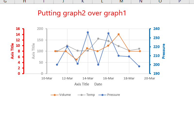
Step 28: Both the graphs are ready now, to overlap each other. Placing graph2 over graph1. The 3 axis graph is ready. 

Step 29: The 3 axis graph is ready, but we see that the lines are overlapping each other which does not give a clear look at the data. To avoid this, you can change the minimum and maximum of the data labels, so that the lines get separated. This can be achieved with hit and trial, try putting different values of minimum and maximum in each axis label and take the best suited. Double click on the data label of graph2. 

Step 30: A Format Axis dialogue box appears. Under the Axis Options, set the minimum and maximum with hit and trial. For example, set the minimum to 0 and maximum to 20. 

Step 31: Similarly Double click, on the secondary axis of graph2. Format Axis dialogue box appears. Under the Axis Options, set the minimum and maximum with hit and trial.  For example, set the minimum to 100 and maximum to 260. 

Step 32: Select both the charts with Ctrl + mouse click. Now, go to Shape Format Tab, and under Arrange section select Group. This helps selecting both graphs as a single entity. 

Step 33: Your three-axis graph is ready.