How to Include Interaction in Regression using R Programming?

In this article, we will look into what is Interaction, and should we use interaction in our model to get better results or not. 

Include Interaction in Regression using R

Let’s say X1 and X2 are features of a dataset and Y is the class label or output that we are trying to predict. Then, If X1 and X2 interact, this means that the effect of X1 on Y depends on the value of X2 and vice versa then where is the interaction between features of the dataset. Now that we know that if our dataset contains interaction or not. We should also know when to take interaction into account in our model for better precision or accuracy. We are going to implement this using the R language.

Should We Include Interaction in Our Model?

There are two questions you should ask before including interaction in your model: 

• Does this interaction make sense conceptually?
• Is the interaction term statistically significant? Or, whether or not we believe the slopes of the regression lines are significantly different.

Implementation in R

Let’s look at the interaction in the linear regression model through an example.

• Dataset
  • Lung Capacity Dataset 
• Parameters/Variables: 
  • Independent Variable(Y): LungCap
  • Dependent Variable(X1): Smoke(Yes/No)
  • Dependent Variable(X2): Age

Example 

Step 1: Load the Data Set

R

# Read in the Lung Cap Data
LungCapData <- read.table(file.choose(),
                          header = T,
                          sep = "\t")

# Attach LungCapData
attach(LungCapData)

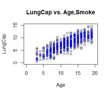
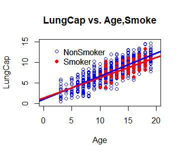
Step 2: Plot the data, using different colors for smoke(red) / non-smoker (blue)

R

# Plot the data, using different
# colours for smoke(red)/non-smoke(blue)
# First, plot the data for
# the Non-Smokers, in Blue
plot(Age[Smoke == "no"],
     LungCap[Smoke == "no"],
     col = "blue",
     ylim = c(0, 15), xlim = c(0, 20),
     xlab = "Age", ylab = "LungCap",
     main = "LungCap vs. Age,Smoke")

Output:

R

# Now, add in the points for
# the Smokers, in Solid Red Circles
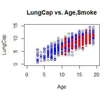
points(Age[Smoke == "yes"],
       LungCap[Smoke == "yes"],
       col = "red", pch = 16)

Output:

R

# And, add in a legend
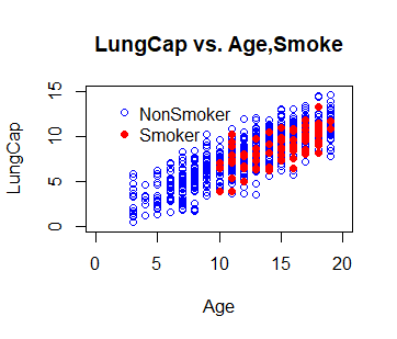
legend(1, 15,
       legend = c("NonSmoker", "Smoker"),
       col = c("blue", "red"),
       pch = c(1, 16), bty = "n")

Output:

Step 3. Fit a Reg Model, using Age, Smoke, and their INTERACTION and Add in the regression lines

R

# Fit a Reg Model, using Age,
# Smoke, and their INTERACTION
model1 <- lm(LungCap ~ Age*Smoke)
coef(model1)

Output:

(Intercept)          Age     Smokeyes Age:Smokeyes 
 1.05157244   0.55823350   0.22601390  -0.05970463

R

# Note, that the "*" fits a model with
# Age, Smoke and AgeXSmoke INT.
# Note, also that the same model
# can be fit using the ":"
model1 <- lm(LungCap ~ Age + Smoke + Age:Smoke)

# Ask for a summary of the model
summary(model1)

Output:

Call:

lm(formula = LungCap ~ Age + Smoke + Age:Smoke)

Residuals:

    Min      1Q  Median      3Q     Max 

-4.8586 -1.0174 -0.0251  1.0004  4.1996 

Coefficients:

             Estimate Std. Error t value Pr(>|t|)    

(Intercept)   1.05157    0.18706   5.622  2.7e-08 ***

Age           0.55823    0.01473  37.885  < 2e-16 ***

Smokeyes      0.22601    1.00755   0.224    0.823    

Age:Smokeyes -0.05970    0.06759  -0.883    0.377    

—

Signif. codes:  0 ‘***’ 0.001 ‘**’ 0.01 ‘*’ 0.05 ‘.’ 0.1 ‘ ’ 1

Residual standard error: 1.515 on 721 degrees of freedom

Multiple R-squared:  0.6776,    Adjusted R-squared:  0.6763 

F-statistic: 505.1 on 3 and 721 DF,  p-value: < 2.2e-16

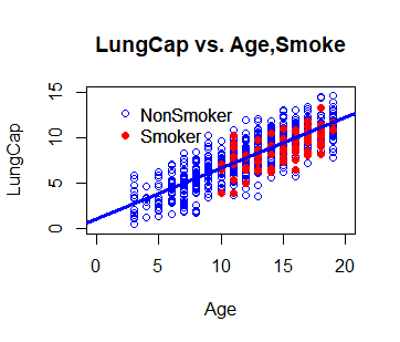
Step 4: Let’s add in the regression lines from our model using the abline command

R

# Now, let's add in the regression
# lines from our mode using the
# abline command for the Non-Smokers, in Blue
abline(a = 1.052, b = 0.558,
       col = "blue", lwd = 3)

Output:

R

# And now, add in the line for Smokers, in Red
abline(a = 1.278, b = 0.498,
       col = "red", lwd = 3)

Output:

R

# Ask for that model summary again
summary(model1)

# Fit the model that does
# NOT include INTERACTION
model2 <- lm(LungCap ~ Age + Smoke)
summary(model2)

Output:

> summary(model1)

Call:
lm(formula = LungCap ~ Age + Smoke + Age:Smoke)

Residuals:
    Min      1Q  Median      3Q     Max 
-4.8586 -1.0174 -0.0251  1.0004  4.1996 

Coefficients:
             Estimate Std. Error t value Pr(>|t|)    
(Intercept)   1.05157    0.18706   5.622  2.7e-08 ***
Age           0.55823    0.01473  37.885  < 2e-16 ***
Smokeyes      0.22601    1.00755   0.224    0.823    
Age:Smokeyes -0.05970    0.06759  -0.883    0.377    
---
Signif. codes:  0 ‘***’ 0.001 ‘**’ 0.01 ‘*’ 0.05 ‘.’ 0.1 ‘ ’ 1

Residual standard error: 1.515 on 721 degrees of freedom
Multiple R-squared:  0.6776,    Adjusted R-squared:  0.6763 
F-statistic: 505.1 on 3 and 721 DF,  p-value: < 2.2e-16

> summary(model2)

Call:
lm(formula = LungCap ~ Age + Smoke)

Residuals:
    Min      1Q  Median      3Q     Max 
-4.8559 -1.0289 -0.0363  1.0083  4.1995 

Coefficients:
            Estimate Std. Error t value Pr(>|t|)    
(Intercept)  1.08572    0.18299   5.933 4.61e-09 ***
Age          0.55540    0.01438  38.628  < 2e-16 ***
Smokeyes    -0.64859    0.18676  -3.473 0.000546 ***
---
Signif. codes:  0 ‘***’ 0.001 ‘**’ 0.01 ‘*’ 0.05 ‘.’ 0.1 ‘ ’ 1

Residual standard error: 1.514 on 722 degrees of freedom
Multiple R-squared:  0.6773,    Adjusted R-squared:  0.6764 
F-statistic: 757.5 on 2 and 722 DF,  p-value: < 2.2e-16