How to implement a gradient descent in Python to find a local minimum ?

Gradient Descent is an iterative algorithm that is used to minimize a function by finding the optimal parameters. Gradient Descent can be applied to any dimension function i.e. 1-D, 2-D, 3-D. In this article, we will be working on finding global minima for parabolic function (2-D) and will be implementing gradient descent in python to find the optimal parameters for the linear regression equation (1-D). Before diving into the implementation part, let us make sure the set of parameters required to implement the gradient descent algorithm. To implement a gradient descent algorithm, we require a cost function that needs to be minimized, the number of iterations, a learning rate to determine the step size at each iteration while moving towards the minimum, partial derivatives for weight & bias to update the parameters at each iteration, and a prediction function. 

Till now we have seen the parameters required for gradient descent. Now let us map the parameters with the gradient descent algorithm and work on an example to better understand gradient descent. Let us consider a parabolic equation y=4x². By looking at the equation we can identify that the parabolic function is minimum at x = 0 i.e. at x=0, y=0. Therefore x=0 is the local minima of the parabolic function y=4x². Now let us see the algorithm for gradient descent and how we can obtain the local minima by applying gradient descent:

Algorithm for Gradient Descent

Steps should be made in proportion to the negative of the function gradient (move away from the gradient) at the current point to find local minima. Gradient Ascent is the procedure for approaching a local maximum of a function by taking steps proportional to the positive of the gradient (moving towards the gradient).

repeat until convergence
{
    w = w - (learning_rate * (dJ/dw))
    b = b - (learning_rate * (dJ/db))
}

Step 1: Initializing all the necessary parameters and deriving the gradient function for the parabolic equation 4x². The derivative of x² is 2x, so the derivative of the parabolic equation 4x² will be 8x. 

x₀ = 3 (random initialization of x)

learning_rate = 0.01 (to determine the step size while moving towards local minima)

gradient =  (Calculating the gradient function)

Step 2: Let us perform 3 iterations of gradient descent:

For each iteration keep on updating the value of x based on the gradient descent formula.

Iteration 1:
    x1 = x0 - (learning_rate * gradient)
    x1 = 3 - (0.01 * (8 * 3))
    x1 = 3 - 0.24
    x1 = 2.76

Iteration 2:
    x2 = x1 - (learning_rate * gradient)
    x2 = 2.76 - (0.01 * (8 * 2.76))
    x2 = 2.76 - 0.2208
    x2 = 2.5392

Iteration 3:
    x3 = x2 - (learning_rate * gradient)
    x3 = 2.5392 - (0.01 * (8 * 2.5392))
    x3 = 2.5392 - 0.203136
    x3 = 2.3360

From the above three iterations of gradient descent, we can notice that the value of x is decreasing iteration by iteration and will slowly converge to 0 (local minima) by running the gradient descent for more iterations. Now you might have a question, for how many iterations we should run gradient descent?

We can set a stopping threshold i.e. when the difference between the previous and the present value of x becomes less than the stopping threshold we stop the iterations. When it comes to the implementation of gradient descent for machine learning algorithms and deep learning algorithms we try to minimize the cost function in the algorithms using gradient descent. Now that we are clear with the gradient descent’s internal working, let us look into the python implementation of gradient descent where we will be minimizing the cost function of the linear regression algorithm and finding the best fit line. In our case the parameters are below mentioned:

Prediction Function

The prediction function for the linear regression algorithm is a linear equation given by y=wx+b. 

prediction_function (y) = (w * x) + b
Here, x is the independent variable
      y is the dependent variable
      w is the weight associated with input variable
      b is the bias

Cost Function

The cost function is used to calculate the loss based on the predictions made. In linear regression, we use mean squared error to calculate the loss. Mean Squared Error is the sum of the squared differences between the actual and predicted values.

Cost Function (J) = 

Here, n is the number of samples

Partial Derivatives (Gradients)

Calculating the partial derivatives for weight and bias using the cost function. We get:

Parameter Updation

Updating the weight and bias by subtracting the multiplication of learning rates and their respective gradients.

w = w - (learning_rate * (dJ/dw))
b = b - (learning_rate * (dJ/db))

Python Implementation for Gradient Descent

In the implementation part, we will be writing two functions, one will be the cost functions that take the actual output and the predicted output as input and returns the loss, the second will be the actual gradient descent function which takes the independent variable, target variable as input and finds the best fit line using gradient descent algorithm. The iterations, learning_rate, and stopping threshold are the tuning parameters for the gradient descent algorithm and can be tuned by the user. In the main function, we will be initializing linearly related random data and applying the gradient descent algorithm on the data to find the best fit line. The optimal weight and bias found by using the gradient descent algorithm are later used to plot the best fit line in the main function. The iterations specify the number of times the update of parameters must be done, the stopping threshold is the minimum change of loss between two successive iterations to stop the gradient descent algorithm.

Python3

# Importing Libraries
import numpy as np
import matplotlib.pyplot as plt

def mean_squared_error(y_true, y_predicted):

    # Calculating the loss or cost
    cost = np.sum((y_true-y_predicted)**2) / len(y_true)
    return cost

# Gradient Descent Function
# Here iterations, learning_rate, stopping_threshold
# are hyperparameters that can be tuned
def gradient_descent(x, y, iterations = 1000, learning_rate = 0.0001,
                     stopping_threshold = 1e-6):

    # Initializing weight, bias, learning rate and iterations
    current_weight = 0.1
    current_bias = 0.01
    iterations = iterations
    learning_rate = learning_rate
    n = float(len(x))

    costs = []
    weights = []
    previous_cost = None

    # Estimation of optimal parameters
    for i in range(iterations):

        # Making predictions
        y_predicted = (current_weight * x) + current_bias

        # Calculating the current cost
        current_cost = mean_squared_error(y, y_predicted)

        # If the change in cost is less than or equal to
        # stopping_threshold we stop the gradient descent
        if previous_cost and abs(previous_cost-current_cost)<=stopping_threshold:
            break

        previous_cost = current_cost

        costs.append(current_cost)
        weights.append(current_weight)

        # Calculating the gradients
        weight_derivative = -(2/n) * sum(x * (y-y_predicted))
        bias_derivative = -(2/n) * sum(y-y_predicted)

        # Updating weights and bias
        current_weight = current_weight - (learning_rate * weight_derivative)
        current_bias = current_bias - (learning_rate * bias_derivative)

        # Printing the parameters for each 1000th iteration
        print(f"Iteration {i+1}: Cost {current_cost}, Weight \
        {current_weight}, Bias {current_bias}")


    # Visualizing the weights and cost at for all iterations
    plt.figure(figsize = (8,6))
    plt.plot(weights, costs)
    plt.scatter(weights, costs, marker='o', color='red')
    plt.title("Cost vs Weights")
    plt.ylabel("Cost")
    plt.xlabel("Weight")
    plt.show()

    return current_weight, current_bias


def main():

    # Data
    X = np.array([32.50234527, 53.42680403, 61.53035803, 47.47563963, 59.81320787,
           55.14218841, 52.21179669, 39.29956669, 48.10504169, 52.55001444,
           45.41973014, 54.35163488, 44.1640495 , 58.16847072, 56.72720806,
           48.95588857, 44.68719623, 60.29732685, 45.61864377, 38.81681754])
    Y = np.array([31.70700585, 68.77759598, 62.5623823 , 71.54663223, 87.23092513,
           78.21151827, 79.64197305, 59.17148932, 75.3312423 , 71.30087989,
           55.16567715, 82.47884676, 62.00892325, 75.39287043, 81.43619216,
           60.72360244, 82.89250373, 97.37989686, 48.84715332, 56.87721319])

    # Estimating weight and bias using gradient descent
    estimated_weight, estimated_bias = gradient_descent(X, Y, iterations=2000)
    print(f"Estimated Weight: {estimated_weight}\nEstimated Bias: {estimated_bias}")

    # Making predictions using estimated parameters
    Y_pred = estimated_weight*X + estimated_bias

    # Plotting the regression line
    plt.figure(figsize = (8,6))
    plt.scatter(X, Y, marker='o', color='red')
    plt.plot([min(X), max(X)], [min(Y_pred), max(Y_pred)], color='blue',markerfacecolor='red',
             markersize=10,linestyle='dashed')
    plt.xlabel("X")
    plt.ylabel("Y")
    plt.show()


if __name__=="__main__":
    main()

Output:

Iteration 1: Cost 4352.088931274409, Weight 0.7593291142562117, Bias 0.02288558130709

Iteration 2: Cost 1114.8561474350017, Weight 1.081602958862324, Bias 0.02918014748569513  

Iteration 3: Cost 341.42912086804455, Weight 1.2391274084945083, Bias 0.03225308846928192 

Iteration 4: Cost 156.64495290904443, Weight 1.3161239281746984, Bias 0.03375132986012604 

Iteration 5: Cost 112.49704004742098, Weight 1.3537591652024805, Bias 0.034479873154934775

Iteration 6: Cost 101.9493925395456, Weight 1.3721549833978113, Bias 0.034832195392868505 

Iteration 7: Cost 99.4293893333546, Weight 1.3811467575154601, Bias 0.03500062439068245   

Iteration 8: Cost 98.82731958262897, Weight 1.3855419247507244, Bias 0.03507916814736111  

Iteration 9: Cost 98.68347500997261, Weight 1.3876903144657764, Bias 0.035113776874486774 

Iteration 10: Cost 98.64910780902792, Weight 1.3887405007983562, Bias 0.035126910596389935

Iteration 11: Cost 98.64089651459352, Weight 1.389253895811451, Bias 0.03512954755833985  

Iteration 12: Cost 98.63893428729509, Weight 1.38950491235671, Bias 0.035127053821718185  

Iteration 13: Cost 98.63846506273883, Weight 1.3896276808137857, Bias 0.035122052266051224

Iteration 14: Cost 98.63835254057648, Weight 1.38968776283053, Bias 0.03511582492978764   

Iteration 15: Cost 98.63832524036214, Weight 1.3897172043139192, Bias 0.03510899846107016 

Iteration 16: Cost 98.63831830104695, Weight 1.389731668997059, Bias 0.035101879159522745 

Iteration 17: Cost 98.63831622628217, Weight 1.389738813163012, Bias 0.03509461674147458  

Estimated Weight: 1.389738813163012

Estimated Bias: 0.03509461674147458

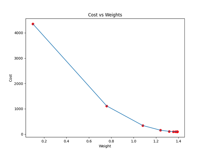
Cost function approaching local minima

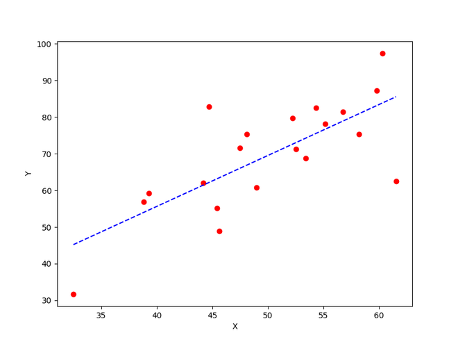
The best fit line obtained using gradient descent