How to Hide Zero Values in Excel

Microsoft Excel enables us to format, organize and calculate data in a spreadsheet. It’s a great tool for preparing datasets and it makes those datasets easier for users and analysts to analyze the data. Sometimes these datasets contain zero values that are not required to be seen. Excel provides an easy way to hide those zero values without affecting the data and the datasets. Whenever we have a large dataset, many of the data values in the dataset may be zero and as per requirement, we may need to hide those zero values and leave the cells empty. Let’s learn how we can Hide Zero Values In Excel.

Hiding Zero Values in Excel

Let’s assume we have the following dataset, showing the sales of different courses in different cities.

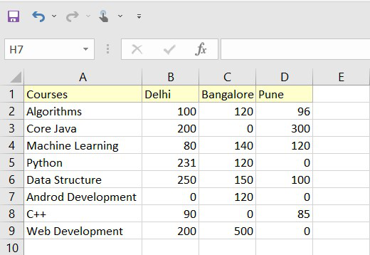
Fig 1 – Dataset

We can see that our dataset contains zero(0) elements that we need to remove. This can be easily done by removing each 0 entry one by one for such a small dataset. But If we have a massive dataset with thousands of entries it became very difficult to remove elements manually.

How to Automatically Hide Zero Values In Cells

In this method, we will use the options provided by Excel to hide zero values in the cells. This method hides the zero value within the complete current worksheet.

Step 1: Open your Excel Sheet and Go to File Tab

Open your dataset sheet and click on the File tab.

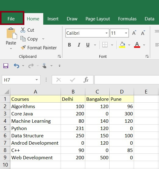
Fig 2 – File Tab

Step 2: Select Options Menu in Side Menu Bar

Once we click the File tab, excel will open the side menu bar. We need to go to the Options menu.

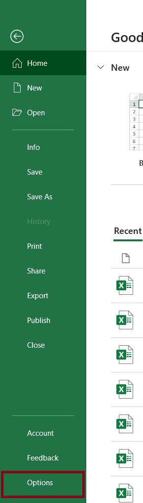
Fig 2 – Option Menu

Step 3: Select Advance

After we click on the Options menu, a popup will come we need to go to the Advance option.

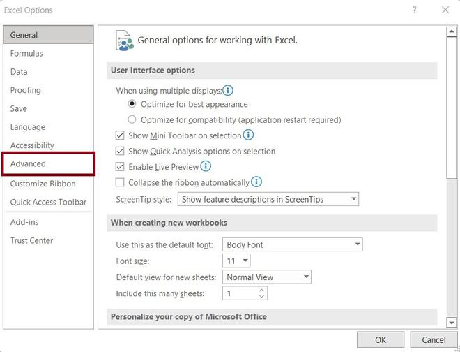
Fig 3 – Advance Option

Step 4: Go to Display Options for this Worksheet and Uncheck Show Row and Columns Headers

In the Advanced options tab, scroll down and go to Display options for this sheet (Here, it is Sheet 4) and uncheck the check box for Show a zero in cells that have zero value and click the OK button.

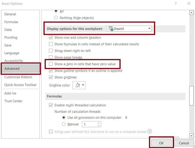
Fig 4 – Display options for the current worksheet

Step 5: Click Ok and Check that Values are Hidden

Once we click on the OK button in the Advanced tab option, excel will automatically hide the zero value in the current working sheet. This change will be also applied to all those cells which zero value as the result of some formula.

Note: This method only hides the zero value, still zero is present in the cell, But it’s hidden.

Fig 5 – Output

Hide Zeores in the Selected Cells Using Conditional Formatting

In this method, we will be using the Conditional Formatting option and setting the rule to hide the zero-value cells in the worksheet. This method is really useful when we want to hide zero values within a specific range. Also, using this method not only we can hide the zero-value cell but we can also highlight the cells which are having zero values.

Step 1: Access the Home Tab and Select Conditional Formatting

Open your dataset sheet and go to Home > Styles > Conditional Formatting > Highlight Cells Rules > Equal To and click on the Equal To option.

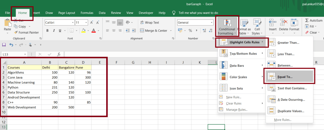
Fig 6 – Home>Conditional Formatting>Highlight Cell Rules> Equal To

Step 2: A Pop Up Box Displayed

Once we click on the Equal To option, it will open a popup asking how we want our zero-value cells.

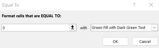
Fig 7- Pop Up Box

In the above picture, we are formatting cells equal to zero with Green color. This formatting rule will fill the zero value cells with green color in the selected dataset. After setting the rules we need to click on the OK button.

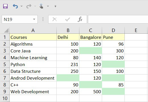
Fig 8 – Output

It also gives flexibility to ultimately make the cells blank by using a custom white color. In the following steps, we can see how we can do that. For this, we need to repeat the first two steps (Step 1 & Step 2) and In step 2 we need to select the Custom Format option.

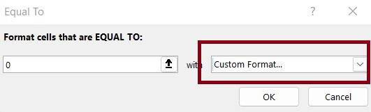
Fig 9 – Custom Format Option

Step 3: Go to Font and Select Colors

Once we click on the OK button, a popup will come we need to go to Font > Color and select a white color.

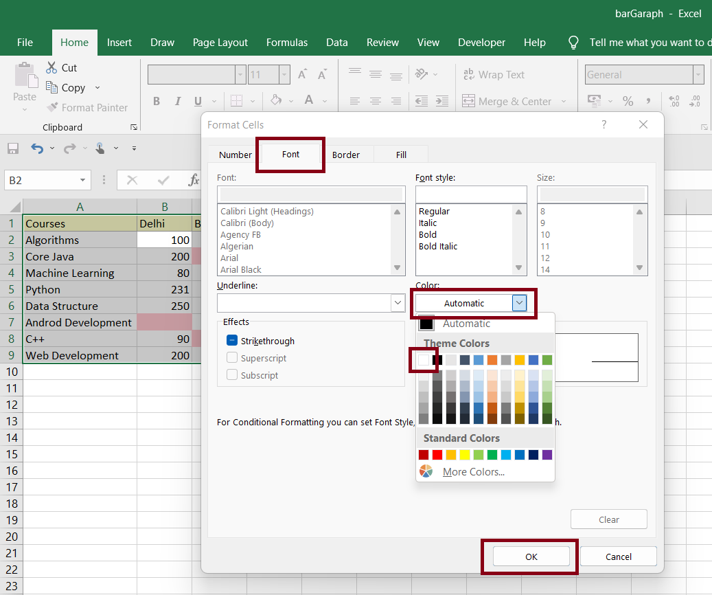
Fig 10 – Font> Colors

Once we click the OK button after selecting our custom color (Here, white) Excel will hide the cells with zero values with a white background.

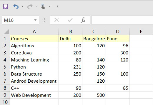
Fig 11 – Output

Hide Zero Values in the Selected Cells Using Format Cells

Follow the below steps to hide Zero Values in the selected cells using Format cells:

Step 1: Select Cells and Select Format Cells

Select the cells or set of cells from where you want to hide zeroes. Now Right-click and select “Format cells”.

Fig 12 – Cells> Format Cells

Step 2: Click on Custom and Enter Custom Type

In the “Format Cells” dialog box, Under Number, click on the “Custom” option and then enter the custom type as “0;-0;;@” and click OK.

Fig 13 – Custom > Enter Custom Type

Step 3: Click Ok and Hide all Zero Values

After clicking Ok you can hide all the zero values within the selected range.

Fig 12- Click Ok

The Custom formatting string “0;-0;;@” is composed of four distinct elements:

The initial “0” is for positive numbers, retaining them in their original state. The subsequent “-0” addresses negative numbers, presenting them as is. And the third element, “0” is absent intentionally to effectively hide zero values. The last element, denoted by “@” symbol, ensures the unaltered display pf text : ;;;.

FAQs on How to Hide the Zero Values in Excel

Why there is need to hide zero values in Excel?

Hiding Zero Values in Excel can improve the readability of your data, especially when dealing with large datasets. It eliminates clutter and makes it easier to focus on the significant data points.

How to hide zero values in a specific cell or range?

Follow the below steps to hide zero value in range:

Step 1: Select the cell range.

Step 2: Right- click and choose “Format cells”.

Step 3: In the “Format cells” dialog box, go to the “Number” tab.

Step 4: Choose “Custom” form the category list.

Step 5: Enter the custom format code “0;-0;;@” in the type field.

Step 6: Click “Ok” to apply the formatting.

How to undo the hidden zero values formatting?

Follow the below steps to undo the hidden zeroes values:

Step 1: Select the cells or range with hidden zero values.

Step 2: Right-click and choose “Format cells”

Step 3: In the “Number” tab, select a different formatting option, such as “General” or “Number”.

Step 4: Click “OK” to apply the new formatting and reveal the hidden zero values.

Will hidden values reappear if we share the Excel file with others?

Yes, hidden zero values will retain their formatting when you share the Excel file with others. However, users can adjust their own settings to reveal or hide zero values according to their preferences.