How to Add, Use and Remove Filter in Excel

Filter in Excel – Easy Steps

1. Select any cell within the range
2. Select Data > Filter
3. Select the column header
4. Click the Filter Icon > Choose a Filter
5. Enter the filter criteria > Click Ok

Working with a database is a crucial job. With every data added increases the comprehensiveness to manage records and pick out the needed information from any corner of the database. Keeping the struggle in mind, Excel is a great tool to store and extract data in a hassle-free manner. It is convenient for every data-driven purpose. The filter option provides efficiency in searching for the needed data from a huge pile of records. Let’s understand what exactly the filter option is. The filter in Excel displays data that is relevant for the users to make decisions. The user applies some criteria and the records get separated wherein required data show up and others disappear. This reduces the burden of scrolling each record to find the best match plus saves a lot of time. Excel filter is the most preferred feature among professionals to rely on when making crucial decisions.

What is Filter in Excel

The filter is a powerful feature of Excel that allows users to sort through and display some specific subsets of data from a larger dataset based on user-defined criteria. When we apply Filter to a column, it creates a small drop-down arrow that appears in the column header. These arrows reveal a list of unique values or numerical values of the column. Users can select specific items to display various filter options to show only the data that meets the chosen data.

How to Filter in Excel

Filter Feature is used to filter the data according to your needs. To filter the data, select the entries to be visible and deselect the rest of the items.

There are three methods to add Filters in Excel mentioned below:

1. With the Filter option under the Data tab.
2. With the Filter option under the Home tab.
3. With the Shortcut key.

How to Filter Data in Excel With Filter Option in Home Tab

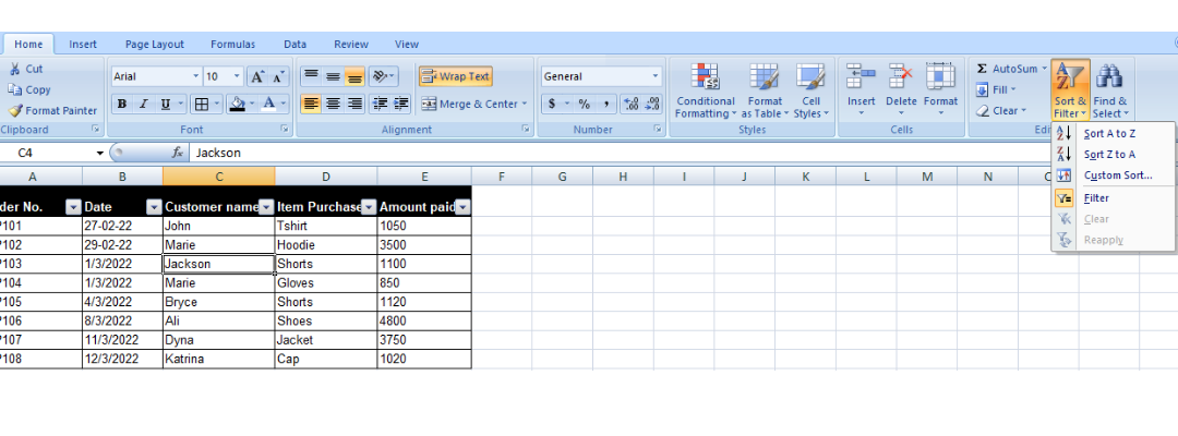
The process begins with the drop-down arrow appearing on the headings of each column. In the Home tab, there is a “Filter” option under the “Sort and Filter” drop-down of the editing section. Follow the below steps to use the Filter tab.

Step 1: Select the Data

Choose the data, then opt for the “Filter” feature within the “Sort and Filter” drop-down menu.

Step 2: Preview Filters

Filters are applied to the chosen data range. The filters are represented by the drop-down arrows, as depicted in the image below.

Step 3: Select any Drop-Down Arrow to View the Filter

Click the drop-down arrow in any column to view all the content of the column.

How to Use Filter Option in Excel in Data Tab

Select a cell from the record. Under the Data tab, there’s an option visible as ‘Filter’. Click on it and you can see the drop drop-down on each column header. 

Shortcut Key for Filtering Data in Excel

Using Keyboard shortcuts to perform any operations helps to speed up daily tasks. Follow the below steps to use Filter in Excel:

Select any cell from the record and simply go with any of these methods:

• Ctrl + Shift + L (Press the keys together)
• Alt + A + T (Press the keys together)

• Learn more about Excel Keyboard Shortcuts

How to Add Filters in Excel Example

To understand the whole mechanism, let’s take an example. The store offers a wide range of apparel for both men and women. The record includes details like the Order Number, Date, Customer Name, Item Purchased, and Amount paid. Filtering the data is never been easy but Excel makes it easy to understand for everyone. To make each concept clear here are some cases for each type of filter option. You can learn to apply them and experiment with options as well.

• Example 1: How to Check the Purchase History of Marie
• Example 2: You need the sales record for 1st March 2022
• Example 3: You want to know the name of the items priced more than 2000
• Example 4: You want to filter the Records by Hoodie and Shorts

If you want to know what all purchases have been made by Marie, you can follow the steps below. This helps in understanding the customer relationship with the business.

Example 1: How to Check the Purchase History of Marie

Step 1: Click on the Drop Down of Customer Name

Click on the arrow near the Customer name  

Step 2: Click on Select All Option

Click on the Select All option.

Step 3: Check on Customer Name “Marie”

The filter is applied to the column which shows the purchase details of Marie.

Example 2: You need the sales record for 1st March 2022

In case you need all the sales made on 1st March 2022, apply custom filter options with each step given below. 

Step 1: Click on the Arrow near the Date

Click on the arrow near the Date. 

Step 2: Hover the cursor on Data Filters

Step 3: Click on Custom Filters

Step 4: Select the Date for which you want to see the Records.

The record for the selected date will appear in the sheet.

Example 3: You want to know the name of the items priced more than 2000

Here, we are going to discuss finding the records with ‘Greater than’ criteria to show up all records above the specified amount.

Step 1: Click on the Arrow near the Amount Paid

Step 2: Hover the cursor on Number Filters and Click on Greater than.

Step 3: Enter the Desired Filtering Amount

Sales records with the amount paid more than 2000 will be displayed.

Example 4: You want to filter the Records by Hoodie and Shorts

In case, you want to apply a filter on two options from the same column. You can do so by selecting desired options from the text filters. Follow the steps below.

Step 1: Click on the arrow near ‘Customer name’.  

Step 2: Click on Select All

Step 3: Check on Hoodie and Shorts.

The filter will show the records related to Item Hoodie and Shorts.

How To Apply Multiple Filters in Excel

You can apply multiple filters to a dataset for better analyzing and extracting relevant information. This feature of applying multiple filters to the dataset is said to be cumulative. Follow the below steps to apply multiple filters:

Step 1: Click the Drop-down Arrow

Click the drop-down arrow of the column which you want to filter (Here we are filtering Item Purchased)

Step 2: Filter Menu will Appear

Step 3: Check or Uncheck the Boxes

Check or Uncheck the boxes of the data you want to Filter, then click OK.

Step 4: Preview the Filters

The Filters are applied to the data.

How To Clear a Filter from Column in Excel

Follow the below steps to Remove the filter after applying it, or clear it from the worksheet so you’ll be able to filter content in different ways.

Step 1: Click the Drop-Down Arrow for the Filter you Want to Remove

Step 2: The Filter menu will Appear

Step 3: Choose Clear Filter From [COLUMN NAME] from the Filter Menu.

Step 4: Preview the Cleared Filter Data

How to Remove Filter in Excel

Step 1: Go to the Data Tab

Step 2: Click on Sort & Filter Group and Click Clear

Step 3: Preview Data

How to Filter by Color in Excel

If you have manually formatted or applied conditional formatting to your worksheet data, you can utilize color-based filtering.

To do this, click on the autofilter drop-down arrow, which will reveal the “Filter by Color” option, offering one or more choices depending on the formatting in each column:

• Filter by Cell Color
• Filter by Font Color
• Filter by Cell Icon

For Example, suppose you’ve formatted cells in a specific column with three different background colors (green, red, and orange), and you want to display only the orange cells. Follow these steps:

Step 1: Click on the Filter Arrow

Click on the Filter Arrow located in the header cell of the column you’re interested.

Step 2: Select the Filter by Color

Step 3: Click on the Desired Color

How to Use Advance Filter

Sometimes Basic Filtering may not give you enough options, If you need a Filter for something specific, you can use Advanced Filtering options.

Excel includes several advanced Filtering tools, such as Search, Text, Date, and number Filtering, which can enhance your result to help you to find exactly what you need.

How to Create a Filtering Search box for Excel Data

Excel has the feature to search for data that contains an exact phrase, number, date, and more. Follow the below steps to filter with Search:

Step 1: Click the drop-down arrow for the Column you Want to Filter

Step 2: The Filter Menu will Appear

Enter a Search term into the Search box. Search results will appear automatically below the Text Filters Field as you type.

Step 3: Preview the Filtered Data

The worksheet will be Filtered according to your Search term.

How To Use Advanced Text Filters

Advanced text filters can be used to display more specific information, like cells that contain a certain number of characters or data that excludes a specific word or number.

Step 1: Click the drop-down Arrow for the Column you want to Filter

Step 2: The Filter menu will Appear

Step 3: Go to the Text Filters

Go to the Text Filters then select the desired text filter from the dropdown menu.

Step 3: Enter the Desrired Text in the Cutsom AutoFilter dialog box

The Custom AutoFilter dialog box will appear. Enter the desired text to the left of the Filter, then click ok.

Step 4: Preview the Filtered Data

The data is now filtered by the selected text filter.

How to Use Advanced Number Filters

Step 1: Click on the Drop-Down Arrow for the Column you want to Filter

Step 2: Preview the Filter Menu

Step 3: Go to the Number Filters

Select the Number Filters and then Select your preferred choice. Here we are choosing Less Than.

Step 4: Select your Preferred Criteria

In the Custom AutoFilter, You can Enter your preferred Value.

Step 5: Preview the Data

FAQs

How to add a Filter to data in Excel?

Follow the below steps to add a filter to the data:

Step 1: Select the dataset.

Step 2: Go to the “Data” tab in the Ribbon.

Step 3: Click on the “Filter” Button in the “Sort & Filter” group.

Step 4: Excel will add filter arrows to the headers of each column.

How to clear or remove filters in Excel?

To remove filters in Excel and display the entire dataset so that you can add other filters to the data:

Step 1: Select the data set with the Filters.

Step 2: Go to the “Data” tab and select the Clear button in the “Sort and Filter” Group.

This will help you to remove all the Filters from your data.

How to apply Filter to a table?

When we convert a range of data to a table, Excel automatically adds filter arrows to the table headers, making it easier to work with filters and analyze the data with more clarity.

How to filter data using the date ranges in Excel?

To filter data using date ranges in Excel follow the below steps:

Step 1: Click on the Filter arrow for the column containing dates.

Step 2: In the drop-down menu, select “Date Filters” and then choose options like “Between”, ETC. Or else you can use “Custom Filter” and specify a date range.